

310
A. S. Semenov
The transformation of the elastic object at runtime is shown in Fig. 21.1 by a
curve, where the unfolded object on the left side of the curve and folded one on the
right side of the curve are presented.
21.2.2 The Analysis of the Capacity Curve
There are many fractal dimensions introduced in mathematical literature, e.g., [19–
21]. Here, the capacity curve is analyzed by the box-counting dimension. The ideas
of the method are the following:
1. Determine curve via boxes covered it.
2. Cover the maximum element of a curve by boxes.
3. Scale only the boxes, do not scale the curve.
Definition 1 Let N be the number of boxes calculated by function n: (δ, ε) → N,
where ε is a grid (a box size) that contains at least one element of the curve δ. If
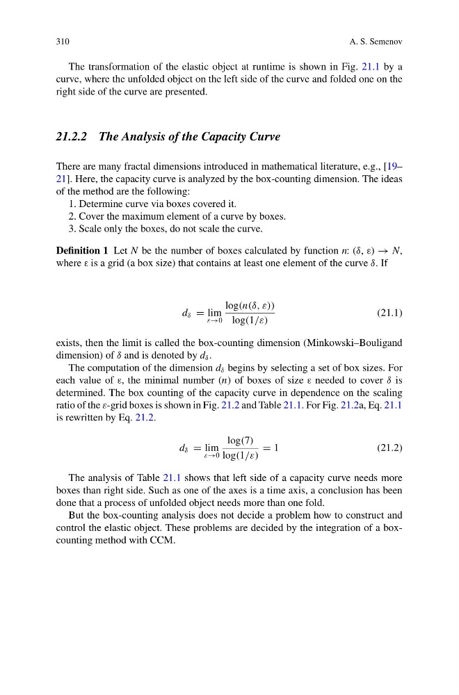
d δ = lim
ε→0
log(n(δ, ε))
log(1/ε)
(21.1)
exists, then the limit is called the box-counting dimension (Minkowski–Bouligand
dimension) of δ and is denoted by d δ .
The computation of the dimension d δ begins by selecting a set of box sizes. For
each value of ε, the minimal number (n) of boxes of size ε needed to cover δ is
determined. The box counting of the capacity curve in dependence on the scaling
ratio of the ε-grid boxes is shown in Fig. 21.2 and Table 21.1. For Fig. 21.2a, Eq. 21.1
is rewritten by Eq. 21.2.
d δ = lim
ε→0
log(7)
log(1/ε)
= 1
(21.2)
The analysis of Table 21.1 shows that left side of a capacity curve needs more
boxes than right side. Such as one of the axes is a time axis, a conclusion has been
done that a process of unfolded object needs more than one fold.
But the box-counting analysis does not decide a problem how to construct and
control the elastic object. These problems are decided by the integration of a boxcounting method with CCM.
A. S. Semenov
The transformation of the elastic object at runtime is shown in Fig. 21.1 by a
curve, where the unfolded object on the left side of the curve and folded one on the
right side of the curve are presented.
21.2.2 The Analysis of the Capacity Curve
There are many fractal dimensions introduced in mathematical literature, e.g., [19–
21]. Here, the capacity curve is analyzed by the box-counting dimension. The ideas
of the method are the following:
1. Determine curve via boxes covered it.
2. Cover the maximum element of a curve by boxes.
3. Scale only the boxes, do not scale the curve.
Definition 1 Let N be the number of boxes calculated by function n: (δ, ε) → N,
where ε is a grid (a box size) that contains at least one element of the curve δ. If
d δ = lim
ε→0
log(n(δ, ε))
log(1/ε)
(21.1)
exists, then the limit is called the box-counting dimension (Minkowski–Bouligand
dimension) of δ and is denoted by d δ .
The computation of the dimension d δ begins by selecting a set of box sizes. For
each value of ε, the minimal number (n) of boxes of size ε needed to cover δ is
determined. The box counting of the capacity curve in dependence on the scaling
ratio of the ε-grid boxes is shown in Fig. 21.2 and Table 21.1. For Fig. 21.2a, Eq. 21.1
is rewritten by Eq. 21.2.
d δ = lim
ε→0
log(7)
log(1/ε)
= 1
(21.2)
The analysis of Table 21.1 shows that left side of a capacity curve needs more
boxes than right side. Such as one of the axes is a time axis, a conclusion has been
done that a process of unfolded object needs more than one fold.
But the box-counting analysis does not decide a problem how to construct and
control the elastic object. These problems are decided by the integration of a boxcounting method with CCM.