

20 Using Spectral Form of Mathematical Description …
301
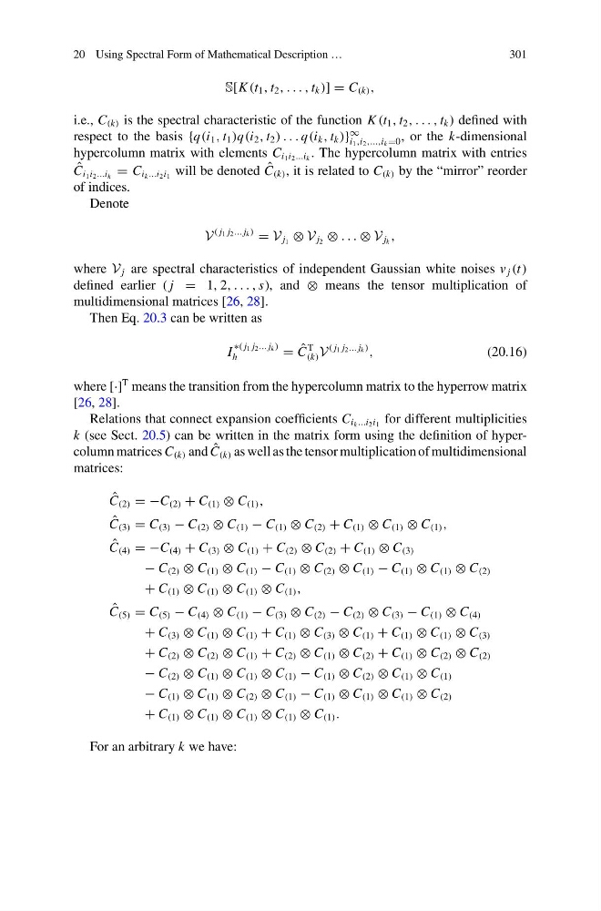
S[K (t 1 , t 2 , . . . , t k )] = C (k) ,
i.e., C (k) is the spectral characteristic of the function K (t 1 , t 2 , . . . , t k ) defined with
respect to the basis {q(i 1 , t 1 )q(i 2 , t 2 ) . . . q(i k , t k )}
∞
i 1 ,i 2 ,...,i k =0 , or the k-dimensional
hypercolumn matrix with elements C i 1 i 2 ...i k . The hypercolumn matrix with entries
ˆ
C i 1 i 2 ...i k = C i k ...i 2 i 1 will be denoted ˆ
C (k) , it is related to C (k) by the “mirror” reorder
of indices.
Denote
V
( j 1 j 2 ... j k )
= V j 1 ⊗ V j 2 ⊗ . . . ⊗ V j k ,
where V j are spectral characteristics of independent Gaussian white noises v j (t)
defined earlier ( j = 1, 2, . . . , s), and ⊗ means the tensor multiplication of
multidimensional matrices [26, 28].
Then Eq. 20.3 can be written as
I
∗( j 1 j 2 ... j k )
h
= ˆ
C
T
(k) V
( j 1 j 2 ... j k )
,
(20.16)
where [·]
T means the transition from the hypercolumn matrix to the hyperrow matrix
[26, 28].
Relations that connect expansion coefficients C i k ...i 2 i 1 for different multiplicities
k (see Sect. 20.5) can be written in the matrix form using the definition of hypercolumn matrices C (k) and ˆ
C (k) as well as the tensor multiplication of multidimensional
matrices:
ˆ
C (2) = −C (2) + C (1) ⊗ C (1) ,
ˆ
C (3) = C (3) − C (2) ⊗ C (1) − C (1) ⊗ C (2) + C (1) ⊗ C (1) ⊗ C (1) ,
ˆ
C (4) = −C (4) + C (3) ⊗ C (1) + C (2) ⊗ C (2) + C (1) ⊗ C (3)
− C (2) ⊗ C (1) ⊗ C (1) − C (1) ⊗ C (2) ⊗ C (1) − C (1) ⊗ C (1) ⊗ C (2)
+ C (1) ⊗ C (1) ⊗ C (1) ⊗ C (1) ,
ˆ
C (5) = C (5) − C (4) ⊗ C (1) − C (3) ⊗ C (2) − C (2) ⊗ C (3) − C (1) ⊗ C (4)
+ C (3) ⊗ C (1) ⊗ C (1) + C (1) ⊗ C (3) ⊗ C (1) + C (1) ⊗ C (1) ⊗ C (3)
+ C (2) ⊗ C (2) ⊗ C (1) + C (2) ⊗ C (1) ⊗ C (2) + C (1) ⊗ C (2) ⊗ C (2)
− C (2) ⊗ C (1) ⊗ C (1) ⊗ C (1) − C (1) ⊗ C (2) ⊗ C (1) ⊗ C (1)
− C (1) ⊗ C (1) ⊗ C (2) ⊗ C (1) − C (1) ⊗ C (1) ⊗ C (1) ⊗ C (2)
+ C (1) ⊗ C (1) ⊗ C (1) ⊗ C (1) ⊗ C (1) .
For an arbitrary k we have:
301
S[K (t 1 , t 2 , . . . , t k )] = C (k) ,
i.e., C (k) is the spectral characteristic of the function K (t 1 , t 2 , . . . , t k ) defined with
respect to the basis {q(i 1 , t 1 )q(i 2 , t 2 ) . . . q(i k , t k )}
∞
i 1 ,i 2 ,...,i k =0 , or the k-dimensional
hypercolumn matrix with elements C i 1 i 2 ...i k . The hypercolumn matrix with entries
ˆ
C i 1 i 2 ...i k = C i k ...i 2 i 1 will be denoted ˆ
C (k) , it is related to C (k) by the “mirror” reorder
of indices.
Denote
V
( j 1 j 2 ... j k )
= V j 1 ⊗ V j 2 ⊗ . . . ⊗ V j k ,
where V j are spectral characteristics of independent Gaussian white noises v j (t)
defined earlier ( j = 1, 2, . . . , s), and ⊗ means the tensor multiplication of
multidimensional matrices [26, 28].
Then Eq. 20.3 can be written as
I
∗( j 1 j 2 ... j k )
h
= ˆ
C
T
(k) V
( j 1 j 2 ... j k )
,
(20.16)
where [·]
T means the transition from the hypercolumn matrix to the hyperrow matrix
[26, 28].
Relations that connect expansion coefficients C i k ...i 2 i 1 for different multiplicities
k (see Sect. 20.5) can be written in the matrix form using the definition of hypercolumn matrices C (k) and ˆ
C (k) as well as the tensor multiplication of multidimensional
matrices:
ˆ
C (2) = −C (2) + C (1) ⊗ C (1) ,
ˆ
C (3) = C (3) − C (2) ⊗ C (1) − C (1) ⊗ C (2) + C (1) ⊗ C (1) ⊗ C (1) ,
ˆ
C (4) = −C (4) + C (3) ⊗ C (1) + C (2) ⊗ C (2) + C (1) ⊗ C (3)
− C (2) ⊗ C (1) ⊗ C (1) − C (1) ⊗ C (2) ⊗ C (1) − C (1) ⊗ C (1) ⊗ C (2)
+ C (1) ⊗ C (1) ⊗ C (1) ⊗ C (1) ,
ˆ
C (5) = C (5) − C (4) ⊗ C (1) − C (3) ⊗ C (2) − C (2) ⊗ C (3) − C (1) ⊗ C (4)
+ C (3) ⊗ C (1) ⊗ C (1) + C (1) ⊗ C (3) ⊗ C (1) + C (1) ⊗ C (1) ⊗ C (3)
+ C (2) ⊗ C (2) ⊗ C (1) + C (2) ⊗ C (1) ⊗ C (2) + C (1) ⊗ C (2) ⊗ C (2)
− C (2) ⊗ C (1) ⊗ C (1) ⊗ C (1) − C (1) ⊗ C (2) ⊗ C (1) ⊗ C (1)
− C (1) ⊗ C (1) ⊗ C (2) ⊗ C (1) − C (1) ⊗ C (1) ⊗ C (1) ⊗ C (2)
+ C (1) ⊗ C (1) ⊗ C (1) ⊗ C (1) ⊗ C (1) .
For an arbitrary k we have: