

296
K. A. Rybakov
variable. This provides simultaneous modeling the set of iterated stochastic integrals
of an arbitrary multiplicity.
20.5 Relations for Expansion Coefficients and Iterated
Stratonovich Stochastic Integrals
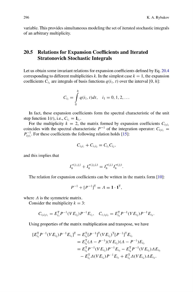
Let us obtain some invariant relations for expansion coefficients defined by Eq. 20.4
corresponding to different multiplicities k. In the simplest case k = 1, the expansion
coefficients C i 1 are integrals of basis functions q(i 1 , t) over the interval [0, h]:
C i 1 =
h
0
q(i 1 , t)dt, i 1 = 0, 1, 2, . . .
In fact, these expansion coefficients form the spectral characteristic of the unit
step function 1(t), i.e., C i 1 = 1 i 1 .
For the multiplicity k = 2, the matrix formed by expansion coefficients C i 2 i 1
coincides with the spectral characteristic P
−1 of the integration operator: C i 2 i 1 =
P
−1
i 2 i 1
. For these coefficients the following relation holds [15]:
C i 2 i 1 + C i 1 i 2 = C i 1 C i 2 ,
and this implies that
I
∗( j 1 j 2 )
h
+ I
∗( j 2 j 1 )
h
= I
∗( j 1 )
h
I
∗( j 2 )
h
.
The relation for expansion coefficients can be written in the matrix form [10]:
P
−1
+ [P
−1
]
T
= Λ = 1 · 1
T
,
where Λ is the symmetric matrix.
Consider the multiplicity k = 3:
C i 3 i 2 i 1 = E
T
i 3
P
−1
(V E i 2 )P
−1 E i 1 , C i 1 i 2 i 3 = E
T
i 1
P
−1
(V E i 2 )P
−1 E i 3 .
Using properties of the matrix multiplication and transpose, we have
[E
T
i 3
P
−1
(V E i 2 )P
−1 E i 1 ]
T
= E
T
i 1
[P
−1
]
T
(V E i 2 )
T
[P
−1
]
T E i 3
= E
T
i 1
(Λ − P
−1
)(V E i 2 )(Λ − P
−1
)E i 3
= E
T
i 1
P
−1
(V E i 2 )P
−1 E i 3 − E
T
i 1
P
−1
(V E i 2 )ΛE i 3
− E
T
i 1
Λ(V E i 2 )P
−1 E i 3 + E
T
i 1
Λ(V E i 2 )ΛE i 3 .
K. A. Rybakov
variable. This provides simultaneous modeling the set of iterated stochastic integrals
of an arbitrary multiplicity.
20.5 Relations for Expansion Coefficients and Iterated
Stratonovich Stochastic Integrals
Let us obtain some invariant relations for expansion coefficients defined by Eq. 20.4
corresponding to different multiplicities k. In the simplest case k = 1, the expansion
coefficients C i 1 are integrals of basis functions q(i 1 , t) over the interval [0, h]:
C i 1 =
h
0
q(i 1 , t)dt, i 1 = 0, 1, 2, . . .
In fact, these expansion coefficients form the spectral characteristic of the unit
step function 1(t), i.e., C i 1 = 1 i 1 .
For the multiplicity k = 2, the matrix formed by expansion coefficients C i 2 i 1
coincides with the spectral characteristic P
−1 of the integration operator: C i 2 i 1 =
P
−1
i 2 i 1
. For these coefficients the following relation holds [15]:
C i 2 i 1 + C i 1 i 2 = C i 1 C i 2 ,
and this implies that
I
∗( j 1 j 2 )
h
+ I
∗( j 2 j 1 )
h
= I
∗( j 1 )
h
I
∗( j 2 )
h
.
The relation for expansion coefficients can be written in the matrix form [10]:
P
−1
+ [P
−1
]
T
= Λ = 1 · 1
T
,
where Λ is the symmetric matrix.
Consider the multiplicity k = 3:
C i 3 i 2 i 1 = E
T
i 3
P
−1
(V E i 2 )P
−1 E i 1 , C i 1 i 2 i 3 = E
T
i 1
P
−1
(V E i 2 )P
−1 E i 3 .
Using properties of the matrix multiplication and transpose, we have
[E
T
i 3
P
−1
(V E i 2 )P
−1 E i 1 ]
T
= E
T
i 1
[P
−1
]
T
(V E i 2 )
T
[P
−1
]
T E i 3
= E
T
i 1
(Λ − P
−1
)(V E i 2 )(Λ − P
−1
)E i 3
= E
T
i 1
P
−1
(V E i 2 )P
−1 E i 3 − E
T
i 1
P
−1
(V E i 2 )ΛE i 3
− E
T
i 1
Λ(V E i 2 )P
−1 E i 3 + E
T
i 1
Λ(V E i 2 )ΛE i 3 .