

20 Using Spectral Form of Mathematical Description …
295
˙
x 2 (t) = x 1 (t)v j 2 (t), x 2 (0) = 0,
. . . . . . . . . . . . . . . . . . . . . . . .
˙
x k (t) = x k−1 (t)v j k (t), x k (0) = 0,
(20.14)
where j 1 , j 2 , . . . , j k = 1, 2, . . . , s and v 1 (t), v 2 (t), …, v s (t) are independent Gaussian white noises corresponding to standard Wiener processes w 1 (t), w 2 (t), …,
w s (t).
This implies that
x k (t) =
t
0
τ k
0
. . .
τ 2
0
dw j 1 (τ 1 ) ◦ dw j 2 (τ 2 ) ◦ . . . ◦ dw j k (τ k ),
x k (h) = I
∗( j 1 j 2 ... j k )
h
,
and the random variables x 1 (h), x 2 (h), …, x k−1 (h) are the iterated Stratonovich
stochastic integrals of multiplicities 1, 2, . . . , k − 1, respectively.
Denote infinite column matrix with entries ζ
( j)
i
by V j . According to [30, 31], V j
are spectral characteristics of independent Gaussian white noises v j (t) corresponding
to Wiener processes w j (t), j = 1, 2, . . . , s.
Consider random processes v j 1 (t), v j 2 (t), …, v j k (t) as input signals of the dynamical system defined by SODE (Eq. 20.8), i.e., g l (t) = v j l (t), l = 1, 2, . . . , k. Then
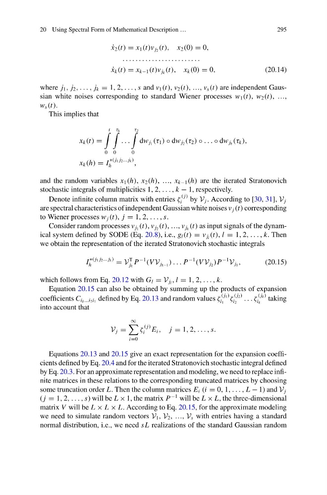
we obtain the representation of the iterated Stratonovich stochastic integrals
I
∗( j 1 j 2 ... j k )
h
= V
T
j k
P
−1
(V V j k−1 ) . . . P
−1
(V V j 2 )P
−1
V j 1 ,
(20.15)
which follows from Eq. 20.12 with G l = V j l , l = 1, 2, . . . , k.
Equation 20.15 can also be obtained by summing up the products of expansion
coefficients C i k ...i 2 i 1 defined by Eq. 20.13 and random values ζ
( j 1 )
i 1
ζ
( j 2 )
i 2
. . . ζ
( j k )
i k
taking
into account that
V j =
∞
i=0
ζ
( j)
i E i , j = 1, 2, . . . , s.
Equations 20.13 and 20.15 give an exact representation for the expansion coefficients defined by Eq. 20.4 and for the iterated Stratonovich stochastic integral defined
by Eq. 20.3. For an approximate representation and modeling, we need to replace infinite matrices in these relations to the corresponding truncated matrices by choosing
some truncation order L. Then the column matrices E i (i = 0, 1, . . . , L − 1) and V j
( j = 1, 2, . . . , s) will be L × 1, the matrix P
−1 will be L × L, the three-dimensional
matrix V will be L × L × L. According to Eq. 20.15, for the approximate modeling
we need to simulate random vectors V 1 , V 2 , …, V s with entries having a standard
normal distribution, i.e., we need s L realizations of the standard Gaussian random
295
˙
x 2 (t) = x 1 (t)v j 2 (t), x 2 (0) = 0,
. . . . . . . . . . . . . . . . . . . . . . . .
˙
x k (t) = x k−1 (t)v j k (t), x k (0) = 0,
(20.14)
where j 1 , j 2 , . . . , j k = 1, 2, . . . , s and v 1 (t), v 2 (t), …, v s (t) are independent Gaussian white noises corresponding to standard Wiener processes w 1 (t), w 2 (t), …,
w s (t).
This implies that
x k (t) =
t
0
τ k
0
. . .
τ 2
0
dw j 1 (τ 1 ) ◦ dw j 2 (τ 2 ) ◦ . . . ◦ dw j k (τ k ),
x k (h) = I
∗( j 1 j 2 ... j k )
h
,
and the random variables x 1 (h), x 2 (h), …, x k−1 (h) are the iterated Stratonovich
stochastic integrals of multiplicities 1, 2, . . . , k − 1, respectively.
Denote infinite column matrix with entries ζ
( j)
i
by V j . According to [30, 31], V j
are spectral characteristics of independent Gaussian white noises v j (t) corresponding
to Wiener processes w j (t), j = 1, 2, . . . , s.
Consider random processes v j 1 (t), v j 2 (t), …, v j k (t) as input signals of the dynamical system defined by SODE (Eq. 20.8), i.e., g l (t) = v j l (t), l = 1, 2, . . . , k. Then
we obtain the representation of the iterated Stratonovich stochastic integrals
I
∗( j 1 j 2 ... j k )
h
= V
T
j k
P
−1
(V V j k−1 ) . . . P
−1
(V V j 2 )P
−1
V j 1 ,
(20.15)
which follows from Eq. 20.12 with G l = V j l , l = 1, 2, . . . , k.
Equation 20.15 can also be obtained by summing up the products of expansion
coefficients C i k ...i 2 i 1 defined by Eq. 20.13 and random values ζ
( j 1 )
i 1
ζ
( j 2 )
i 2
. . . ζ
( j k )
i k
taking
into account that
V j =
∞
i=0
ζ
( j)
i E i , j = 1, 2, . . . , s.
Equations 20.13 and 20.15 give an exact representation for the expansion coefficients defined by Eq. 20.4 and for the iterated Stratonovich stochastic integral defined
by Eq. 20.3. For an approximate representation and modeling, we need to replace infinite matrices in these relations to the corresponding truncated matrices by choosing
some truncation order L. Then the column matrices E i (i = 0, 1, . . . , L − 1) and V j
( j = 1, 2, . . . , s) will be L × 1, the matrix P
−1 will be L × L, the three-dimensional
matrix V will be L × L × L. According to Eq. 20.15, for the approximate modeling
we need to simulate random vectors V 1 , V 2 , …, V s with entries having a standard
normal distribution, i.e., we need s L realizations of the standard Gaussian random