

290
K. A. Rybakov
I
∗( j 1 j 2 ... j k )
h
=
∞
i k =0
. . .
∞
i 2 =0
∞
i 1 =0
C i k ...i 2 i 1 ζ
( j 1 )
i 1
ζ
( j 2 )
i 2
. . . ζ
( j k )
i k
,
(20.3)
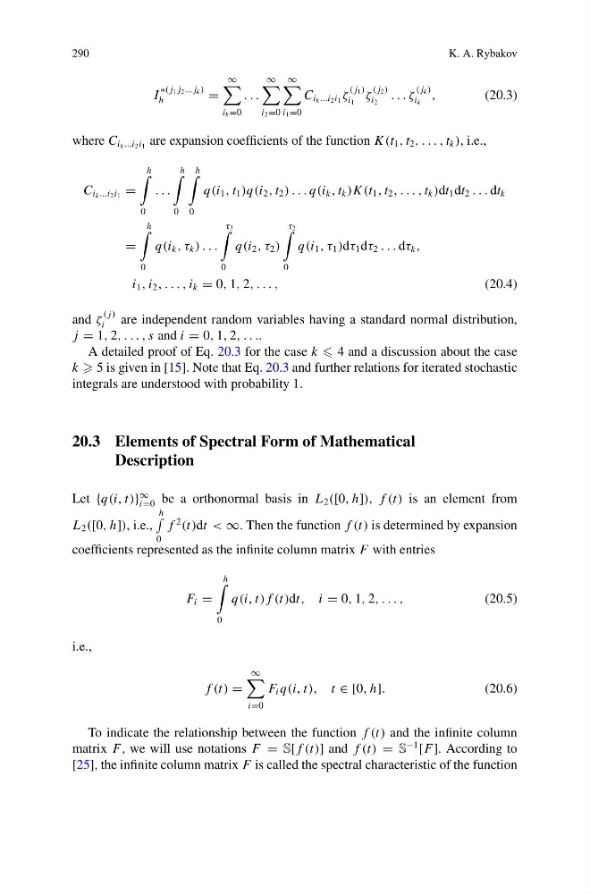
where C i k ...i 2 i 1 are expansion coefficients of the function K (t 1 , t 2 , . . . , t k ), i.e.,
C i k ...i 2 i 1 =
h
0
. . .
h
0
h
0
q(i 1 , t 1 )q(i 2 , t 2 ) . . . q(i k , t k )K (t 1 , t 2 , . . . , t k )dt 1 dt 2 . . . dt k
=
h
0
q(i k , τ k ) . . .
τ 3
0
q(i 2 , τ 2 )
τ 2
0
q(i 1 , τ 1 )dτ 1 dτ 2 . . . dτ k ,
i 1 , i 2 , . . . , i k = 0, 1, 2, . . . ,
(20.4)
and ζ
( j)
i
are independent random variables having a standard normal distribution,
j = 1, 2, . . . , s and i = 0, 1, 2, . . ..
A detailed proof of Eq. 20.3 for the case k 4 and a discussion about the case
k 5 is given in [15]. Note that Eq. 20.3 and further relations for iterated stochastic
integrals are understood with probability 1.
20.3 Elements of Spectral Form of Mathematical
Description
Let {q(i, t)}
∞
i=0 be a orthonormal basis in L 2 ([0, h]), f (t) is an element from
L 2 ([0, h]), i.e.,
h
0
f
2
(t)dt < ∞. Then the function f (t) is determined by expansion
coefficients represented as the infinite column matrix F with entries
F i =
h
0
q(i, t) f (t)dt, i = 0, 1, 2, . . . ,
(20.5)
i.e.,
f (t) =
∞
i=0
F i q(i, t), t ∈ [0, h].
(20.6)
To indicate the relationship between the function f (t) and the infinite column
matrix F, we will use notations F = S[ f (t)] and f (t) = S
−1
[F]. According to
[25], the infinite column matrix F is called the spectral characteristic of the function
K. A. Rybakov
I
∗( j 1 j 2 ... j k )
h
=
∞
i k =0
. . .
∞
i 2 =0
∞
i 1 =0
C i k ...i 2 i 1 ζ
( j 1 )
i 1
ζ
( j 2 )
i 2
. . . ζ
( j k )
i k
,
(20.3)
where C i k ...i 2 i 1 are expansion coefficients of the function K (t 1 , t 2 , . . . , t k ), i.e.,
C i k ...i 2 i 1 =
h
0
. . .
h
0
h
0
q(i 1 , t 1 )q(i 2 , t 2 ) . . . q(i k , t k )K (t 1 , t 2 , . . . , t k )dt 1 dt 2 . . . dt k
=
h
0
q(i k , τ k ) . . .
τ 3
0
q(i 2 , τ 2 )
τ 2
0
q(i 1 , τ 1 )dτ 1 dτ 2 . . . dτ k ,
i 1 , i 2 , . . . , i k = 0, 1, 2, . . . ,
(20.4)
and ζ
( j)
i
are independent random variables having a standard normal distribution,
j = 1, 2, . . . , s and i = 0, 1, 2, . . ..
A detailed proof of Eq. 20.3 for the case k 4 and a discussion about the case
k 5 is given in [15]. Note that Eq. 20.3 and further relations for iterated stochastic
integrals are understood with probability 1.
20.3 Elements of Spectral Form of Mathematical
Description
Let {q(i, t)}
∞
i=0 be a orthonormal basis in L 2 ([0, h]), f (t) is an element from
L 2 ([0, h]), i.e.,
h
0
f
2
(t)dt < ∞. Then the function f (t) is determined by expansion
coefficients represented as the infinite column matrix F with entries
F i =
h
0
q(i, t) f (t)dt, i = 0, 1, 2, . . . ,
(20.5)
i.e.,
f (t) =
∞
i=0
F i q(i, t), t ∈ [0, h].
(20.6)
To indicate the relationship between the function f (t) and the infinite column
matrix F, we will use notations F = S[ f (t)] and f (t) = S
−1
[F]. According to
[25], the infinite column matrix F is called the spectral characteristic of the function