

284
A. Yu. Morozov and D. L. Reviznikov
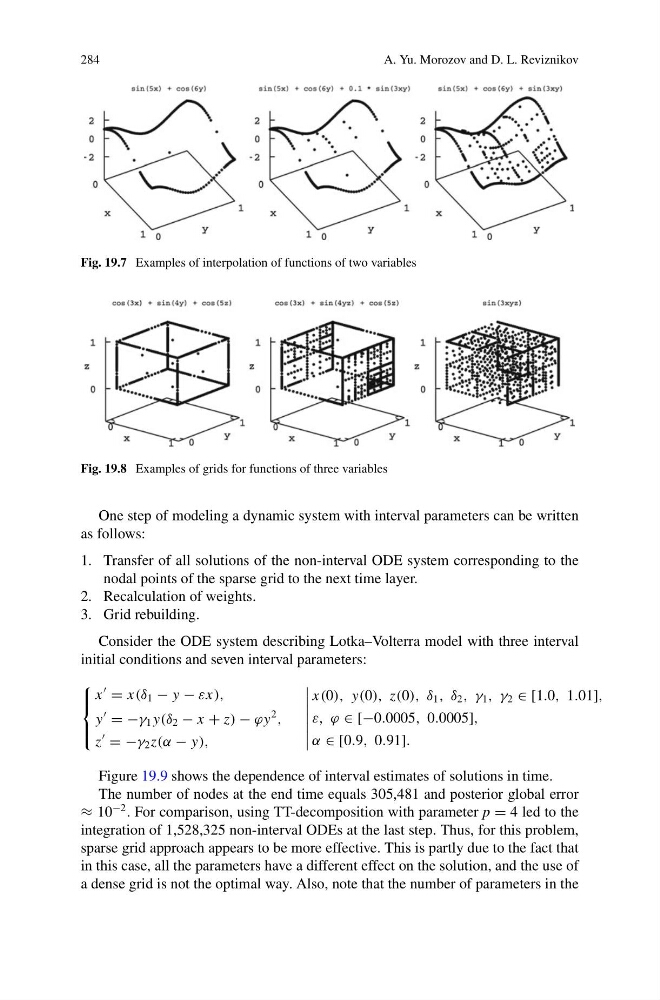
Fig. 19.7 Examples of interpolation of functions of two variables
Fig. 19.8 Examples of grids for functions of three variables
One step of modeling a dynamic system with interval parameters can be written
as follows:
1. Transfer of all solutions of the non-interval ODE system corresponding to the
nodal points of the sparse grid to the next time layer.
2. Recalculation of weights.
3. Grid rebuilding.
Consider the ODE system describing Lotka–Volterra model with three interval
initial conditions and seven interval parameters:
⎧
⎪ ⎨
⎪ ⎩
x
= x(δ 1 − y − εx),
y
= −γ 1 y(δ 2 − x + z) − ϕy
2
,
z
= −γ 2 z(α − y),
x(0), y(0), z(0), δ 1 , δ 2 , γ 1 , γ 2 ∈ [1.0, 1.01],
ε, ϕ ∈ [−0.0005, 0.0005],
α ∈ [0.9, 0.91].
Figure 19.9 shows the dependence of interval estimates of solutions in time.
The number of nodes at the end time equals 305,481 and posterior global error
≈ 10
−2 . For comparison, using TT-decomposition with parameter p = 4 led to the
integration of 1,528,325 non-interval ODEs at the last step. Thus, for this problem,
sparse grid approach appears to be more effective. This is partly due to the fact that
in this case, all the parameters have a different effect on the solution, and the use of
a dense grid is not the optimal way. Also, note that the number of parameters in the
A. Yu. Morozov and D. L. Reviznikov
Fig. 19.7 Examples of interpolation of functions of two variables
Fig. 19.8 Examples of grids for functions of three variables
One step of modeling a dynamic system with interval parameters can be written
as follows:
1. Transfer of all solutions of the non-interval ODE system corresponding to the
nodal points of the sparse grid to the next time layer.
2. Recalculation of weights.
3. Grid rebuilding.
Consider the ODE system describing Lotka–Volterra model with three interval
initial conditions and seven interval parameters:
⎧
⎪ ⎨
⎪ ⎩
x
= x(δ 1 − y − εx),
y
= −γ 1 y(δ 2 − x + z) − ϕy
2
,
z
= −γ 2 z(α − y),
x(0), y(0), z(0), δ 1 , δ 2 , γ 1 , γ 2 ∈ [1.0, 1.01],
ε, ϕ ∈ [−0.0005, 0.0005],
α ∈ [0.9, 0.91].
Figure 19.9 shows the dependence of interval estimates of solutions in time.
The number of nodes at the end time equals 305,481 and posterior global error
≈ 10
−2 . For comparison, using TT-decomposition with parameter p = 4 led to the
integration of 1,528,325 non-interval ODEs at the last step. Thus, for this problem,
sparse grid approach appears to be more effective. This is partly due to the fact that
in this case, all the parameters have a different effect on the solution, and the use of
a dense grid is not the optimal way. Also, note that the number of parameters in the