

15 Astronomical and Geophysical Factors of the Perturbed Chandler Wobble …
211
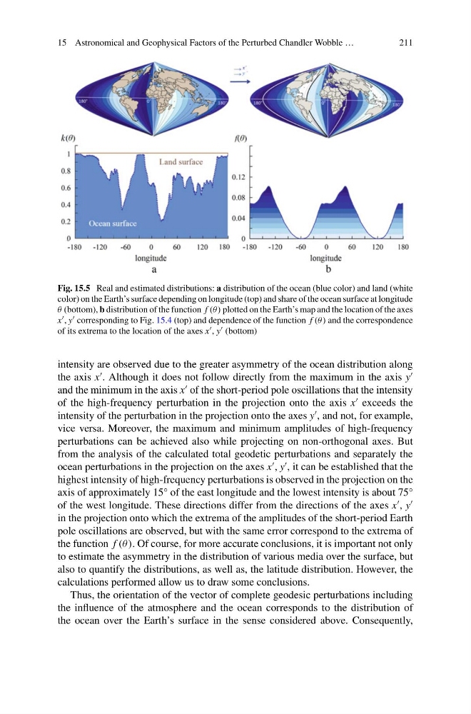
Fig. 15.5 Real and estimated distributions: a distribution of the ocean (blue color) and land (white
color) on the Earth’s surface depending on longitude (top) and share of the ocean surface at longitude
θ (bottom), b distribution of the function f (θ) plotted on the Earth’s map and the location of the axes
x , y corresponding to Fig. 15.4 (top) and dependence of the function f (θ) and the correspondence
of its extrema to the location of the axes x , y (bottom)
intensity are observed due to the greater asymmetry of the ocean distribution along
the axis x
. Although it does not follow directly from the maximum in the axis y
and the minimum in the axis x
of the short-period pole oscillations that the intensity
of the high-frequency perturbation in the projection onto the axis x
exceeds the
intensity of the perturbation in the projection onto the axes y
, and not, for example,
vice versa. Moreover, the maximum and minimum amplitudes of high-frequency
perturbations can be achieved also while projecting on non-orthogonal axes. But
from the analysis of the calculated total geodetic perturbations and separately the
ocean perturbations in the projection on the axes x
, y
, it can be established that the
highest intensity of high-frequency perturbations is observed in the projection on the
axis of approximately 15° of the east longitude and the lowest intensity is about 75°
of the west longitude. These directions differ from the directions of the axes x
, y
in the projection onto which the extrema of the amplitudes of the short-period Earth
pole oscillations are observed, but with the same error correspond to the extrema of
the function f (θ ). Of course, for more accurate conclusions, it is important not only
to estimate the asymmetry in the distribution of various media over the surface, but
also to quantify the distributions, as well as, the latitude distribution. However, the
calculations performed allow us to draw some conclusions.
Thus, the orientation of the vector of complete geodesic perturbations including
the influence of the atmosphere and the ocean corresponds to the distribution of
the ocean over the Earth’s surface in the sense considered above. Consequently,
211
Fig. 15.5 Real and estimated distributions: a distribution of the ocean (blue color) and land (white
color) on the Earth’s surface depending on longitude (top) and share of the ocean surface at longitude
θ (bottom), b distribution of the function f (θ) plotted on the Earth’s map and the location of the axes
x , y corresponding to Fig. 15.4 (top) and dependence of the function f (θ) and the correspondence
of its extrema to the location of the axes x , y (bottom)
intensity are observed due to the greater asymmetry of the ocean distribution along
the axis x
. Although it does not follow directly from the maximum in the axis y
and the minimum in the axis x
of the short-period pole oscillations that the intensity
of the high-frequency perturbation in the projection onto the axis x
exceeds the
intensity of the perturbation in the projection onto the axes y
, and not, for example,
vice versa. Moreover, the maximum and minimum amplitudes of high-frequency
perturbations can be achieved also while projecting on non-orthogonal axes. But
from the analysis of the calculated total geodetic perturbations and separately the
ocean perturbations in the projection on the axes x
, y
, it can be established that the
highest intensity of high-frequency perturbations is observed in the projection on the
axis of approximately 15° of the east longitude and the lowest intensity is about 75°
of the west longitude. These directions differ from the directions of the axes x
, y
in the projection onto which the extrema of the amplitudes of the short-period Earth
pole oscillations are observed, but with the same error correspond to the extrema of
the function f (θ ). Of course, for more accurate conclusions, it is important not only
to estimate the asymmetry in the distribution of various media over the surface, but
also to quantify the distributions, as well as, the latitude distribution. However, the
calculations performed allow us to draw some conclusions.
Thus, the orientation of the vector of complete geodesic perturbations including
the influence of the atmosphere and the ocean corresponds to the distribution of
the ocean over the Earth’s surface in the sense considered above. Consequently,