

162
I. S. Nikitin et al.
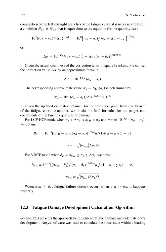
conjugation of the left and right branches of the fatigue curve, it is necessary to fulfill
a condition N LH = N VH that is equivalent to the equation for the quantity σ :
10
3 [(σ B − σ u )/σ ]
1/β LH = 10
8
(σ u − ˜
σ u )
σ u + σ − ˜
σ u
1/β VH
or
σ = 10
−5β LH (σ B − σ u )
1 + σ/(σ u − ˜
σ u )
β LH /β VH .
Given the actual smallness of the correction term in square brackets, one can set
the correction value σ by an approximate formula:
σ = 10
−5β LH (σ B − σ u ).
The corresponding approximate value N ∗ = N LH (σ ∗ ) is determined by
N ∗ = 10
3 [(σ B − σ u )//σ ]
1/β LH ≈ 10
8
.
Given the updated estimates obtained for the transition point from one branch
of the fatigue curve to another, we obtain the final formulas for the ranges and
coefficients of the kinetic equations of damage.
For LCF-HCF mode when σ u + σ u < σ LH < σ B and σ = 10
−5β LH (σ B − σ u ),
we obtain:
B LH = 10
−3 [σ LH − σ u /(σ B − σ u )]
1/β LH α/(1 + α − γ )/(1 − γ ),
σ L H =
σ 1 max
σ 1 /2.
For VHCF mode when ˜
σ u < σ V H ≤ σ u + σ u , we have:
B VH = 10
−8
σ VH − ˜
σ u
(σ u − ˜
σ u )
1/β V H α
(1 + α − γ )/(1 − γ ),
σ VH =
σ 1 max
σ 1 /2.
When σ VH ≤ ˜
σ u , fatigue failure doesn’t occur; when σ LH ≥ σ B , it happens
instantly.
12.3 Fatigue Damage Development Calculation Algorithm
Section 12.3 presents the approach to implement fatigue damage and calculate one’s
development. Ansys software was used to calculate the stress state within a loading
I. S. Nikitin et al.
conjugation of the left and right branches of the fatigue curve, it is necessary to fulfill
a condition N LH = N VH that is equivalent to the equation for the quantity σ :
10
3 [(σ B − σ u )/σ ]
1/β LH = 10
8
(σ u − ˜
σ u )
σ u + σ − ˜
σ u
1/β VH
or
σ = 10
−5β LH (σ B − σ u )
1 + σ/(σ u − ˜
σ u )
β LH /β VH .
Given the actual smallness of the correction term in square brackets, one can set
the correction value σ by an approximate formula:
σ = 10
−5β LH (σ B − σ u ).
The corresponding approximate value N ∗ = N LH (σ ∗ ) is determined by
N ∗ = 10
3 [(σ B − σ u )//σ ]
1/β LH ≈ 10
8
.
Given the updated estimates obtained for the transition point from one branch
of the fatigue curve to another, we obtain the final formulas for the ranges and
coefficients of the kinetic equations of damage.
For LCF-HCF mode when σ u + σ u < σ LH < σ B and σ = 10
−5β LH (σ B − σ u ),
we obtain:
B LH = 10
−3 [σ LH − σ u /(σ B − σ u )]
1/β LH α/(1 + α − γ )/(1 − γ ),
σ L H =
σ 1 max
σ 1 /2.
For VHCF mode when ˜
σ u < σ V H ≤ σ u + σ u , we have:
B VH = 10
−8
σ VH − ˜
σ u
(σ u − ˜
σ u )
1/β V H α
(1 + α − γ )/(1 − γ ),
σ VH =
σ 1 max
σ 1 /2.
When σ VH ≤ ˜
σ u , fatigue failure doesn’t occur; when σ LH ≥ σ B , it happens
instantly.
12.3 Fatigue Damage Development Calculation Algorithm
Section 12.3 presents the approach to implement fatigue damage and calculate one’s
development. Ansys software was used to calculate the stress state within a loading