

1.3 Fluid Dynamics
27
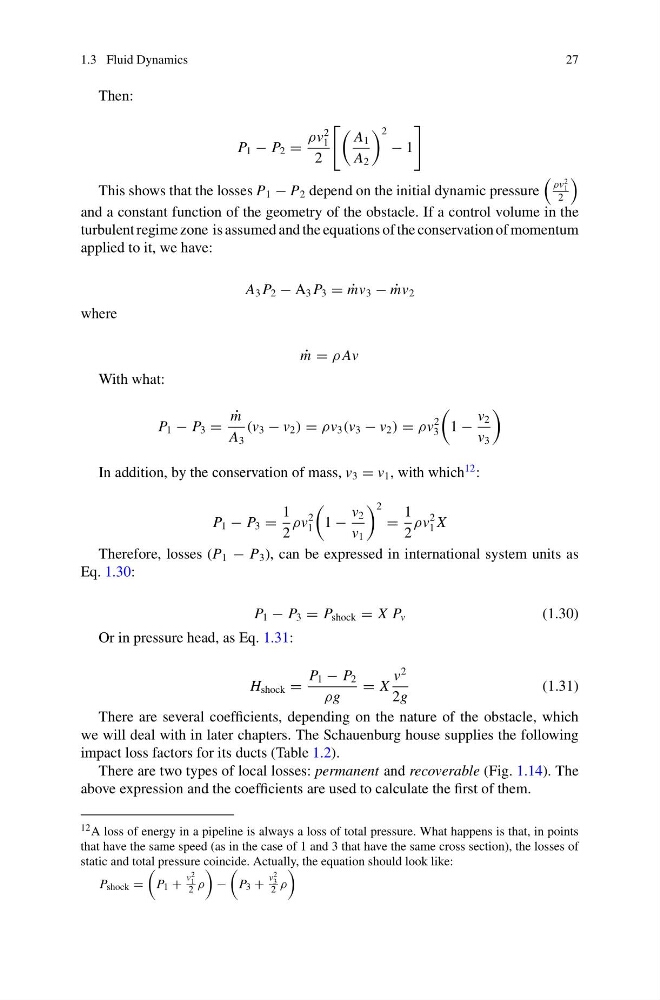
Then:
P 1 − P 2 =
ρv
2
1
2
A 1
A 2
2
− 1
This shows that the losses P 1 − P 2 depend on the initial dynamic pressure
ρv
2
1
2
and a constant function of the geometry of the obstacle. If a control volume in the
turbulent regime zone is assumed and the equations of the conservation of momentum
applied to it, we have:
A 3 P 2 − A 3 P 3 = ˙
mv 3 − ˙
mv 2
where
˙
m = ρ Av
With what:
P 1 − P 3 =
˙
m
A 3
(v 3 − v 2 ) = ρv 3 (v 3 − v 2 ) = ρv
2
3
1 −
v 2
v 3
In addition, by the conservation of mass, v 3 = v 1 , with which
12 :
P 1 − P 3 =
1
2
ρv
2
1
1 −
v 2
v 1
2
=
1
2
ρv
2
1 X
Therefore, losses (P 1 − P 3 ), can be expressed in international system units as
Eq. 1.30:
P 1 − P 3 = P shock = X P v
(1.30)
Or in pressure head, as Eq. 1.31:
H shock =
P 1 − P 2
ρg
= X
v
2
2g
(1.31)
There are several coefficients, depending on the nature of the obstacle, which
we will deal with in later chapters. The Schauenburg house supplies the following
impact loss factors for its ducts (Table 1.2).
There are two types of local losses: permanent and recoverable (Fig. 1.14). The
above expression and the coefficients are used to calculate the first of them.
12 A loss of energy in a pipeline is always a loss of total pressure. What happens is that, in points
that have the same speed (as in the case of 1 and 3 that have the same cross section), the losses of
static and total pressure coincide. Actually, the equation should look like:
P shock =
P 1 +
v 2
1
2 ρ
−
P 3 +
v 2
3
2 ρ
27
Then:
P 1 − P 2 =
ρv
2
1
2
A 1
A 2
2
− 1
This shows that the losses P 1 − P 2 depend on the initial dynamic pressure
ρv
2
1
2
and a constant function of the geometry of the obstacle. If a control volume in the
turbulent regime zone is assumed and the equations of the conservation of momentum
applied to it, we have:
A 3 P 2 − A 3 P 3 = ˙
mv 3 − ˙
mv 2
where
˙
m = ρ Av
With what:
P 1 − P 3 =
˙
m
A 3
(v 3 − v 2 ) = ρv 3 (v 3 − v 2 ) = ρv
2
3
1 −
v 2
v 3
In addition, by the conservation of mass, v 3 = v 1 , with which
12 :
P 1 − P 3 =
1
2
ρv
2
1
1 −
v 2
v 1
2
=
1
2
ρv
2
1 X
Therefore, losses (P 1 − P 3 ), can be expressed in international system units as
Eq. 1.30:
P 1 − P 3 = P shock = X P v
(1.30)
Or in pressure head, as Eq. 1.31:
H shock =
P 1 − P 2
ρg
= X
v
2
2g
(1.31)
There are several coefficients, depending on the nature of the obstacle, which
we will deal with in later chapters. The Schauenburg house supplies the following
impact loss factors for its ducts (Table 1.2).
There are two types of local losses: permanent and recoverable (Fig. 1.14). The
above expression and the coefficients are used to calculate the first of them.
12 A loss of energy in a pipeline is always a loss of total pressure. What happens is that, in points
that have the same speed (as in the case of 1 and 3 that have the same cross section), the losses of
static and total pressure coincide. Actually, the equation should look like:
P shock =
P 1 +
v 2
1
2 ρ
−
P 3 +
v 2
3
2 ρ