

8.18 Sizing the Auxiliary Fan
357
Also, as A 1 = A 2, the air velocity along the duct remains constant.
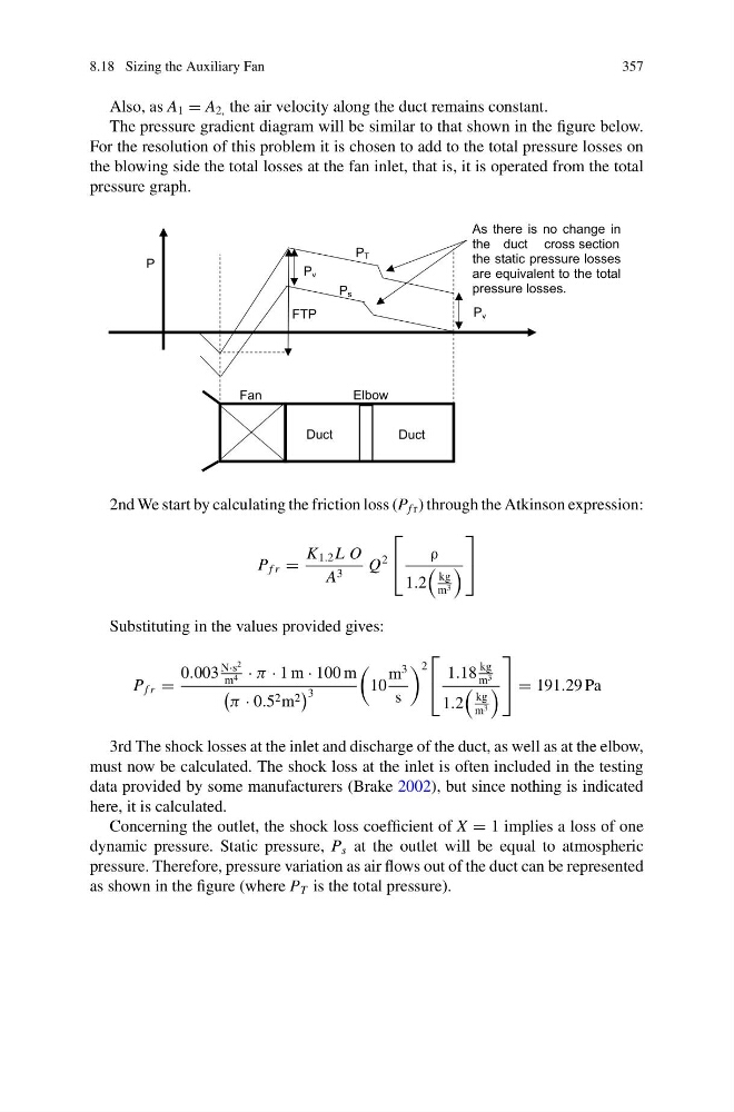
The pressure gradient diagram will be similar to that shown in the figure below.
For the resolution of this problem it is chosen to add to the total pressure losses on
the blowing side the total losses at the fan inlet, that is, it is operated from the total
pressure graph.
P T
P s
FTP
P
P v
Elbow
Duct
Duct
P v
As there is no change in
the duct cross section
the static pressure losses
are equivalent to the total
pressure losses.
Fan
2nd We start by calculating the friction loss (P f r ) through the Atkinson expression:
P f r =
K 1.2 L O
A 3
Q
2
⎡
⎣
ρ
1.2
kg
m 3
⎤
⎦
Substituting in the values provided gives:
P f r =
0.003
N·s
2
m 4 · π · 1 m · 100 m
π · 0.5 2 m 2
3
10
m
3
s
2
⎡
⎣
1.18
kg
m 3
1.2
kg
m 3
⎤
⎦ = 191.29 Pa
3rd The shock losses at the inlet and discharge of the duct, as well as at the elbow,
must now be calculated. The shock loss at the inlet is often included in the testing
data provided by some manufacturers (Brake 2002), but since nothing is indicated
here, it is calculated.
Concerning the outlet, the shock loss coefficient of X = 1 implies a loss of one
dynamic pressure. Static pressure, P s at the outlet will be equal to atmospheric
pressure. Therefore, pressure variation as air flows out of the duct can be represented
as shown in the figure (where P T is the total pressure).
357
Also, as A 1 = A 2, the air velocity along the duct remains constant.
The pressure gradient diagram will be similar to that shown in the figure below.
For the resolution of this problem it is chosen to add to the total pressure losses on
the blowing side the total losses at the fan inlet, that is, it is operated from the total
pressure graph.
P T
P s
FTP
P
P v
Elbow
Duct
Duct
P v
As there is no change in
the duct cross section
the static pressure losses
are equivalent to the total
pressure losses.
Fan
2nd We start by calculating the friction loss (P f r ) through the Atkinson expression:
P f r =
K 1.2 L O
A 3
Q
2
⎡
⎣
ρ
1.2
kg
m 3
⎤
⎦
Substituting in the values provided gives:
P f r =
0.003
N·s
2
m 4 · π · 1 m · 100 m
π · 0.5 2 m 2
3
10
m
3
s
2
⎡
⎣
1.18
kg
m 3
1.2
kg
m 3
⎤
⎦ = 191.29 Pa
3rd The shock losses at the inlet and discharge of the duct, as well as at the elbow,
must now be calculated. The shock loss at the inlet is often included in the testing
data provided by some manufacturers (Brake 2002), but since nothing is indicated
here, it is calculated.
Concerning the outlet, the shock loss coefficient of X = 1 implies a loss of one
dynamic pressure. Static pressure, P s at the outlet will be equal to atmospheric
pressure. Therefore, pressure variation as air flows out of the duct can be represented
as shown in the figure (where P T is the total pressure).