

350
8 Secondary Ventilation
(b)
Using the nomogram in Fig. 8.16: 9 m s
−1 .
(c)
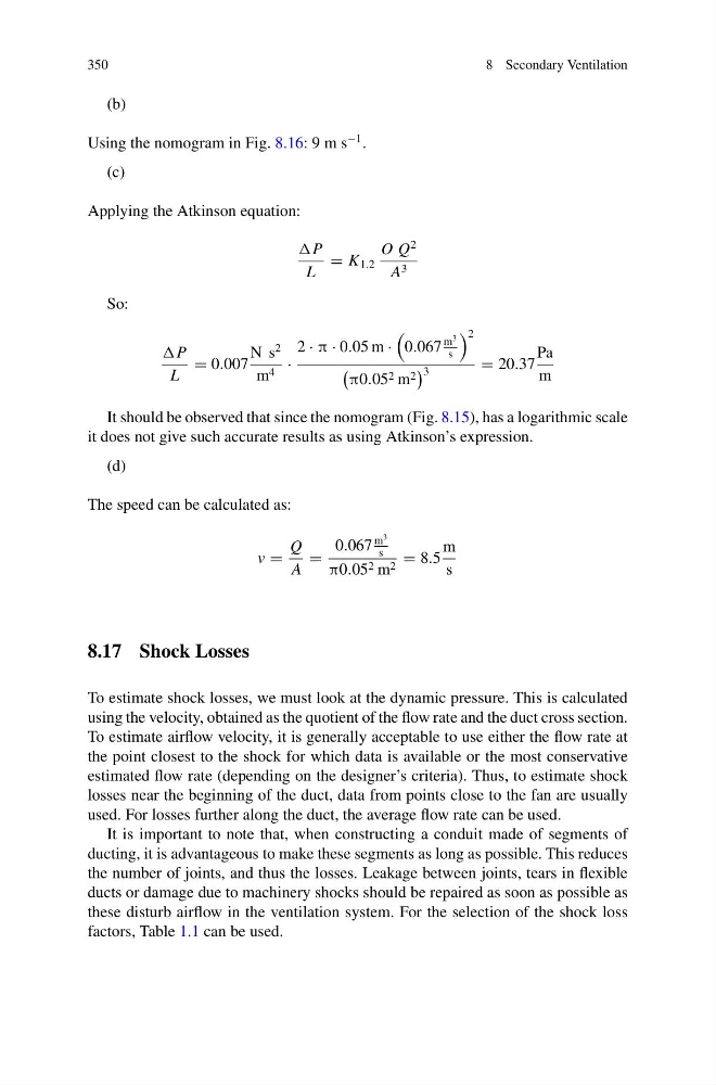
Applying the Atkinson equation:
P
L
= K 1.2
O Q
2
A 3
So:
P
L
= 0.007
N s
2
m 4 ·
2 · π · 0.05 m ·
0.067
m
3
s
2
π0.05 2 m 2
3
= 20.37
Pa
m
It should be observed that since the nomogram (Fig. 8.15), has a logarithmic scale
it does not give such accurate results as using Atkinson’s expression.
(d)
The speed can be calculated as:
v =
Q
A
=
0.067
m
3
s
π0.05 2 m 2 = 8.5
m
s
8.17 Shock Losses
To estimate shock losses, we must look at the dynamic pressure. This is calculated
using the velocity, obtained as the quotient of the flow rate and the duct cross section.
To estimate airflow velocity, it is generally acceptable to use either the flow rate at
the point closest to the shock for which data is available or the most conservative
estimated flow rate (depending on the designer’s criteria). Thus, to estimate shock
losses near the beginning of the duct, data from points close to the fan are usually
used. For losses further along the duct, the average flow rate can be used.
It is important to note that, when constructing a conduit made of segments of
ducting, it is advantageous to make these segments as long as possible. This reduces
the number of joints, and thus the losses. Leakage between joints, tears in flexible
ducts or damage due to machinery shocks should be repaired as soon as possible as
these disturb airflow in the ventilation system. For the selection of the shock loss
factors, Table 1.1 can be used.
8 Secondary Ventilation
(b)
Using the nomogram in Fig. 8.16: 9 m s
−1 .
(c)
Applying the Atkinson equation:
P
L
= K 1.2
O Q
2
A 3
So:
P
L
= 0.007
N s
2
m 4 ·
2 · π · 0.05 m ·
0.067
m
3
s
2
π0.05 2 m 2
3
= 20.37
Pa
m
It should be observed that since the nomogram (Fig. 8.15), has a logarithmic scale
it does not give such accurate results as using Atkinson’s expression.
(d)
The speed can be calculated as:
v =
Q
A
=
0.067
m
3
s
π0.05 2 m 2 = 8.5
m
s
8.17 Shock Losses
To estimate shock losses, we must look at the dynamic pressure. This is calculated
using the velocity, obtained as the quotient of the flow rate and the duct cross section.
To estimate airflow velocity, it is generally acceptable to use either the flow rate at
the point closest to the shock for which data is available or the most conservative
estimated flow rate (depending on the designer’s criteria). Thus, to estimate shock
losses near the beginning of the duct, data from points close to the fan are usually
used. For losses further along the duct, the average flow rate can be used.
It is important to note that, when constructing a conduit made of segments of
ducting, it is advantageous to make these segments as long as possible. This reduces
the number of joints, and thus the losses. Leakage between joints, tears in flexible
ducts or damage due to machinery shocks should be repaired as soon as possible as
these disturb airflow in the ventilation system. For the selection of the shock loss
factors, Table 1.1 can be used.