

1.3 Fluid Dynamics
21
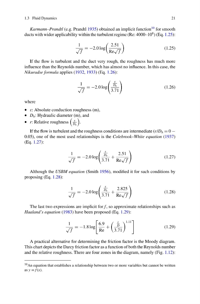
Karmann–Prandtl (e.g. Prandtl 1935) obtained an implicit function
10 for smooth
ducts with wider applicability within the turbulent regime (Re: 4000–10
8 ) (Eq. 1.25):
1
√
f
= −2.0 log
2.51
Re
√
f
(1.25)
If the flow is turbulent and the duct very rough, the roughness has much more
influence than the Reynolds number, which has almost no influence. In this case, the
Nikuradse formula applies (1932, 1933) (Eq. 1.26):
1
√
f
= −2.0 log
ε
D h
3.71
(1.26)
where
• E: Absolute conduction roughness (m),
• D h : Hydraulic diameter (m), and
• r: Relative roughness
ε
D h
.
If the flow is turbulent and the roughness conditions are intermediate (ε/D h = 0 −
0.05), one of the most used relationships is the Colebrook–White equation (1937)
(Eq. 1.27):
1
√
f
= −2.0 log
ε
D h
3.71
+
2.51
Re
√
f
(1.27)
Although the USBM equation (Smith 1956), modified it for such conditions by
proposing (Eq. 1.28):
1
√
f
= −2.0 log
ε
D h
3.71
+
2.825
Re
√
f
(1.28)
The last two expressions are implicit for f , so approximate relationships such as
Haaland’s equation (1983) have been proposed (Eq. 1.29):
1
√
f
= −1.8 log
6.9
Re
+
ε
D
3.71
1.11
(1.29)
A practical alternative for determining the friction factor is the Moody diagram.
This chart depicts the Darcy friction factor as a function of both the Reynolds number
and the relative roughness. There are four zones in the diagram, namely (Fig. 1.12):
10 An equation that establishes a relationship between two or more variables but cannot be written
as y = f (x).
21
Karmann–Prandtl (e.g. Prandtl 1935) obtained an implicit function
10 for smooth
ducts with wider applicability within the turbulent regime (Re: 4000–10
8 ) (Eq. 1.25):
1
√
f
= −2.0 log
2.51
Re
√
f
(1.25)
If the flow is turbulent and the duct very rough, the roughness has much more
influence than the Reynolds number, which has almost no influence. In this case, the
Nikuradse formula applies (1932, 1933) (Eq. 1.26):
1
√
f
= −2.0 log
ε
D h
3.71
(1.26)
where
• E: Absolute conduction roughness (m),
• D h : Hydraulic diameter (m), and
• r: Relative roughness
ε
D h
.
If the flow is turbulent and the roughness conditions are intermediate (ε/D h = 0 −
0.05), one of the most used relationships is the Colebrook–White equation (1937)
(Eq. 1.27):
1
√
f
= −2.0 log
ε
D h
3.71
+
2.51
Re
√
f
(1.27)
Although the USBM equation (Smith 1956), modified it for such conditions by
proposing (Eq. 1.28):
1
√
f
= −2.0 log
ε
D h
3.71
+
2.825
Re
√
f
(1.28)
The last two expressions are implicit for f , so approximate relationships such as
Haaland’s equation (1983) have been proposed (Eq. 1.29):
1
√
f
= −1.8 log
6.9
Re
+
ε
D
3.71
1.11
(1.29)
A practical alternative for determining the friction factor is the Moody diagram.
This chart depicts the Darcy friction factor as a function of both the Reynolds number
and the relative roughness. There are four zones in the diagram, namely (Fig. 1.12):
10 An equation that establishes a relationship between two or more variables but cannot be written
as y = f (x).