

150
4 Mine Ventilation Networks
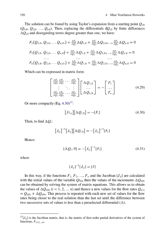
The solution can be found by using Taylor’s expansion from a starting point Q i,0
(Q 1,0 , Q 2,0 , …, Q n,0 ). Then, replacing the differentials dQ i,0 by finite differences
Q i,0 and disregarding terms degree greater than one, we have:
F 1
Q 1,0 , Q 2,0 , . . . Q n,0 ,
+
∂ F 1
∂ Q 1
Q 1,0 +
∂ F 1
∂ Q 2
Q 2,0+···+
∂ F 1
∂ Q n
Q n,0 = 0
F 2
Q 1,0 , Q 2,0 , . . . Q n,0
+
∂ F 2
∂ Q 1
Q 1,0 +
∂ F 2
∂ Q 2
Q 2,0+···+
∂ F 2
∂ Q n
Q n,0 = 0
. . .
. . .
. . .
F n
Q 1,0 , Q 2,0 , . . . Q n,0 ,
+
∂ F n
∂ Q 1
Q 1,0 +
∂ F n
∂ Q 2
Q 2,0+···+
∂ F n
∂ Q n
Q n,0 = 0
Which can be expressed in matrix form:
⎡
⎢
⎢
⎣
∂ F 1
∂ Q 1
∂ F 1
∂ Q 2
· · ·
∂ F 1
∂ Q n
. . .
. . .
. . .
∂ F n
∂ Q 1
∂ F n
∂ Q 2
· · ·
∂ F n
∂ Q n
⎤
⎥
⎥
⎦
⎡
⎣
Q 1,0
. . .
Q n,0
⎤
⎦ = −
⎡
⎣
F 1
. . .
F n
⎤
⎦
(4.29)
Or more compactly (Eq. 4.30)
17 :
J i i j
Q i,0
= −[F i ]
(4.30)
Then, to find Q i :
J i j
−1
J i j
Q i,0
= −
J i j
−1 [F i ]
Hence:
[Q i , 0] = −
J i j
−1 [F i ]
(4.31)
where
[J i j ]
−1
[J i j ] = [I ]
In this way, if the functions F 1, F 2 , …, F n and the Jacobian [J ij ] are calculated
with the initial values of the variable Qi (0) then the values of the increments Q i(0)
can be obtained by solving the system of matrix equations. This allows us to obtain
the values of Q i(0) (i = 1, 2, … n) and thence a new values for the flow rates Q i(1)
= Q i(0) + Q i(0) . This process is repeated with each new set of values for the flow
rates being closer to the real solution than the last set until the difference between
two successive sets of values is less than a preselected differential ().
17 [J ij ] is the Jacobian matrix, that is, the matrix of first-order partial derivatives of the system of
functions, F (1,2…n) .
4 Mine Ventilation Networks
The solution can be found by using Taylor’s expansion from a starting point Q i,0
(Q 1,0 , Q 2,0 , …, Q n,0 ). Then, replacing the differentials dQ i,0 by finite differences
Q i,0 and disregarding terms degree greater than one, we have:
F 1
Q 1,0 , Q 2,0 , . . . Q n,0 ,
+
∂ F 1
∂ Q 1
Q 1,0 +
∂ F 1
∂ Q 2
Q 2,0+···+
∂ F 1
∂ Q n
Q n,0 = 0
F 2
Q 1,0 , Q 2,0 , . . . Q n,0
+
∂ F 2
∂ Q 1
Q 1,0 +
∂ F 2
∂ Q 2
Q 2,0+···+
∂ F 2
∂ Q n
Q n,0 = 0
. . .
. . .
. . .
F n
Q 1,0 , Q 2,0 , . . . Q n,0 ,
+
∂ F n
∂ Q 1
Q 1,0 +
∂ F n
∂ Q 2
Q 2,0+···+
∂ F n
∂ Q n
Q n,0 = 0
Which can be expressed in matrix form:
⎡
⎢
⎢
⎣
∂ F 1
∂ Q 1
∂ F 1
∂ Q 2
· · ·
∂ F 1
∂ Q n
. . .
. . .
. . .
∂ F n
∂ Q 1
∂ F n
∂ Q 2
· · ·
∂ F n
∂ Q n
⎤
⎥
⎥
⎦
⎡
⎣
Q 1,0
. . .
Q n,0
⎤
⎦ = −
⎡
⎣
F 1
. . .
F n
⎤
⎦
(4.29)
Or more compactly (Eq. 4.30)
17 :
J i i j
Q i,0
= −[F i ]
(4.30)
Then, to find Q i :
J i j
−1
J i j
Q i,0
= −
J i j
−1 [F i ]
Hence:
[Q i , 0] = −
J i j
−1 [F i ]
(4.31)
where
[J i j ]
−1
[J i j ] = [I ]
In this way, if the functions F 1, F 2 , …, F n and the Jacobian [J ij ] are calculated
with the initial values of the variable Qi (0) then the values of the increments Q i(0)
can be obtained by solving the system of matrix equations. This allows us to obtain
the values of Q i(0) (i = 1, 2, … n) and thence a new values for the flow rates Q i(1)
= Q i(0) + Q i(0) . This process is repeated with each new set of values for the flow
rates being closer to the real solution than the last set until the difference between
two successive sets of values is less than a preselected differential ().
17 [J ij ] is the Jacobian matrix, that is, the matrix of first-order partial derivatives of the system of
functions, F (1,2…n) .