

4.10 Complex Networks
149
(continued)
N 2
0
1
−1
0
−1
=
0
N 3
0
0
0
−1
1
=
150
M 1
27.7271
24.2047
5.1241
0
0
=
0
M 2
0
0
−5.1241
12.5825 8.7087
=
0
Inverse matrix
Solution
0.50542
0.07367
0.04354 0.01784
0.00346 Q 14(20) = −69.282
−0.49458
0.07367
0.04354 0.01784
0.00346 Q 12(20) =
80.718
−0.39864 −0.74664 −0.44124 0.01438 −0.03507 Q 24(20) =
−6.390
−0.09594 −0.17969 −0.51522 0.00346
0.03853 Q 34(20) = −62.892
−0.09594 −0.17969
0.48478 0.00346
0.03853 Q 23(20) =
87.108
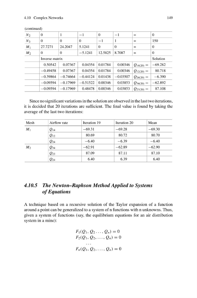
Since no significant variations in the solution are observed in the last two iterations,
it is decided that 20 iterations are sufficient. The final value is found by taking the
average of the last two iterations:
Mesh
Airflow rate
Iteration 19
Iteration 20
Mean
M 1
Q 14
−69.31
−69.28
−69.30
Q 12
80.69
80.72
80.70
Q 24
−6.40
−6.39
−6.40
M 2
Q 34
−62.91
−62.89
−62.90
Q 23
87.09
87.11
87.10
Q 24
6.40
6.39
6.40
4.10.5 The Newton–Raphson Method Applied to Systems
of Equations
A technique based on a recursive solution of the Taylor expansion of a function
around a point can be generalized to a system of n functions with n unknowns. Thus,
given a system of functions (say, the equilibrium equations for an air distribution
system in a mine):
F 1 (Q 1 , Q 2 . . . , Q n ) = 0
F 2 (Q 1 , Q 2 , . . . , Q n ) = 0
. . .
F n (Q 1 , Q 2 , . . . , Q n ) = 0
149
(continued)
N 2
0
1
−1
0
−1
=
0
N 3
0
0
0
−1
1
=
150
M 1
27.7271
24.2047
5.1241
0
0
=
0
M 2
0
0
−5.1241
12.5825 8.7087
=
0
Inverse matrix
Solution
0.50542
0.07367
0.04354 0.01784
0.00346 Q 14(20) = −69.282
−0.49458
0.07367
0.04354 0.01784
0.00346 Q 12(20) =
80.718
−0.39864 −0.74664 −0.44124 0.01438 −0.03507 Q 24(20) =
−6.390
−0.09594 −0.17969 −0.51522 0.00346
0.03853 Q 34(20) = −62.892
−0.09594 −0.17969
0.48478 0.00346
0.03853 Q 23(20) =
87.108
Since no significant variations in the solution are observed in the last two iterations,
it is decided that 20 iterations are sufficient. The final value is found by taking the
average of the last two iterations:
Mesh
Airflow rate
Iteration 19
Iteration 20
Mean
M 1
Q 14
−69.31
−69.28
−69.30
Q 12
80.69
80.72
80.70
Q 24
−6.40
−6.39
−6.40
M 2
Q 34
−62.91
−62.89
−62.90
Q 23
87.09
87.11
87.10
Q 24
6.40
6.39
6.40
4.10.5 The Newton–Raphson Method Applied to Systems
of Equations
A technique based on a recursive solution of the Taylor expansion of a function
around a point can be generalized to a system of n functions with n unknowns. Thus,
given a system of functions (say, the equilibrium equations for an air distribution
system in a mine):
F 1 (Q 1 , Q 2 . . . , Q n ) = 0
F 2 (Q 1 , Q 2 , . . . , Q n ) = 0
. . .
F n (Q 1 , Q 2 , . . . , Q n ) = 0