

4.10 Complex Networks
145
In other words, it is a linear equation in Q i , which allows, together with the mass
conservation equations, forms a system of linear equations where the number of
equations is equal to the number of unknowns, and is, therefore, solvable.
The procedure is then repeated substituting the value calculated for Q i(1) into the
above equation. Consequently, for the second iteration we have:
P i(2) =
R i Q i(1)
Q i(2)
Which gives us the system of linear equations for the second iteration.
For those branches whose calculated R i Q i(n) is lower than the real one (initially
unknown) the method will correct them to a higher flow rate (lower resistance implies
greater flow rate). The reverse is also true: for those branches whose calculated R i Q i(n)
is higher than the actual one, the system will correct to a lower flow rate. Successive
iterations compensate for these deviations. It is, therefore, advisable that, from the
second iteration onwards, the starting flow rate for the nth iteration be calculated
as the average of the previous two values for Q i .
16 This procedure has the joint
advantages of converging quickly to the final solution, and of not needing to assume
an initial distribution of flows. In addition, as opposed to the Hardy–Cross method,
corrections in this method are made to individual branches rather than meshes.
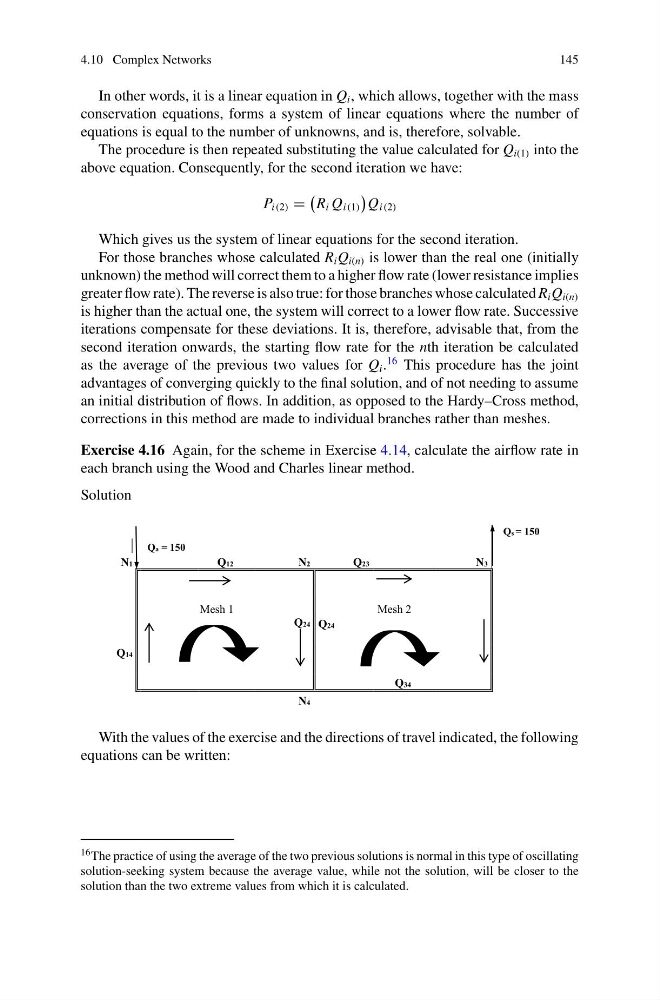
Exercise 4.16 Again, for the scheme in Exercise 4.14, calculate the airflow rate in
each branch using the Wood and Charles linear method.
Solution
Qa = 150
Qs = 150
N1
Q12
N 2
Q23
N3
Mesh 1
Mesh 2
Q24 Q24
Q14
Q34
N4
With the values of the exercise and the directions of travel indicated, the following
equations can be written:
16 The practice of using the average of the two previous solutions is normal in this type of oscillating
solution-seeking system because the average value, while not the solution, will be closer to the
solution than the two extreme values from which it is calculated.
145
In other words, it is a linear equation in Q i , which allows, together with the mass
conservation equations, forms a system of linear equations where the number of
equations is equal to the number of unknowns, and is, therefore, solvable.
The procedure is then repeated substituting the value calculated for Q i(1) into the
above equation. Consequently, for the second iteration we have:
P i(2) =
R i Q i(1)
Q i(2)
Which gives us the system of linear equations for the second iteration.
For those branches whose calculated R i Q i(n) is lower than the real one (initially
unknown) the method will correct them to a higher flow rate (lower resistance implies
greater flow rate). The reverse is also true: for those branches whose calculated R i Q i(n)
is higher than the actual one, the system will correct to a lower flow rate. Successive
iterations compensate for these deviations. It is, therefore, advisable that, from the
second iteration onwards, the starting flow rate for the nth iteration be calculated
as the average of the previous two values for Q i .
16 This procedure has the joint
advantages of converging quickly to the final solution, and of not needing to assume
an initial distribution of flows. In addition, as opposed to the Hardy–Cross method,
corrections in this method are made to individual branches rather than meshes.
Exercise 4.16 Again, for the scheme in Exercise 4.14, calculate the airflow rate in
each branch using the Wood and Charles linear method.
Solution
Qa = 150
Qs = 150
N1
Q12
N 2
Q23
N3
Mesh 1
Mesh 2
Q24 Q24
Q14
Q34
N4
With the values of the exercise and the directions of travel indicated, the following
equations can be written:
16 The practice of using the average of the two previous solutions is normal in this type of oscillating
solution-seeking system because the average value, while not the solution, will be closer to the
solution than the two extreme values from which it is calculated.