

57
2.1 Aerofoils
the average velocity in a channel, as obtained in a one-dimensional analysis. This
product has the correct order of magnitude, but the exact result depends on the distribution of the shear stress and the velocity gradient across a channel section. With
a trapezoidal velocity profile and with an infinitesimally thin transition from core to
wall, it follows that the energy dissipation integral (Eq. 2.9) equals the product of
the velocity in the flow core and the shear stress at the wall.
The reasoning based on the energy Eq. (2.7) and the work Eq. (2.8) demonstrates
that the wall friction affects the entire boundary layer. Energy dissipation by friction
is thus no local phenomenon. Moreover, the dissipation continues downstream of
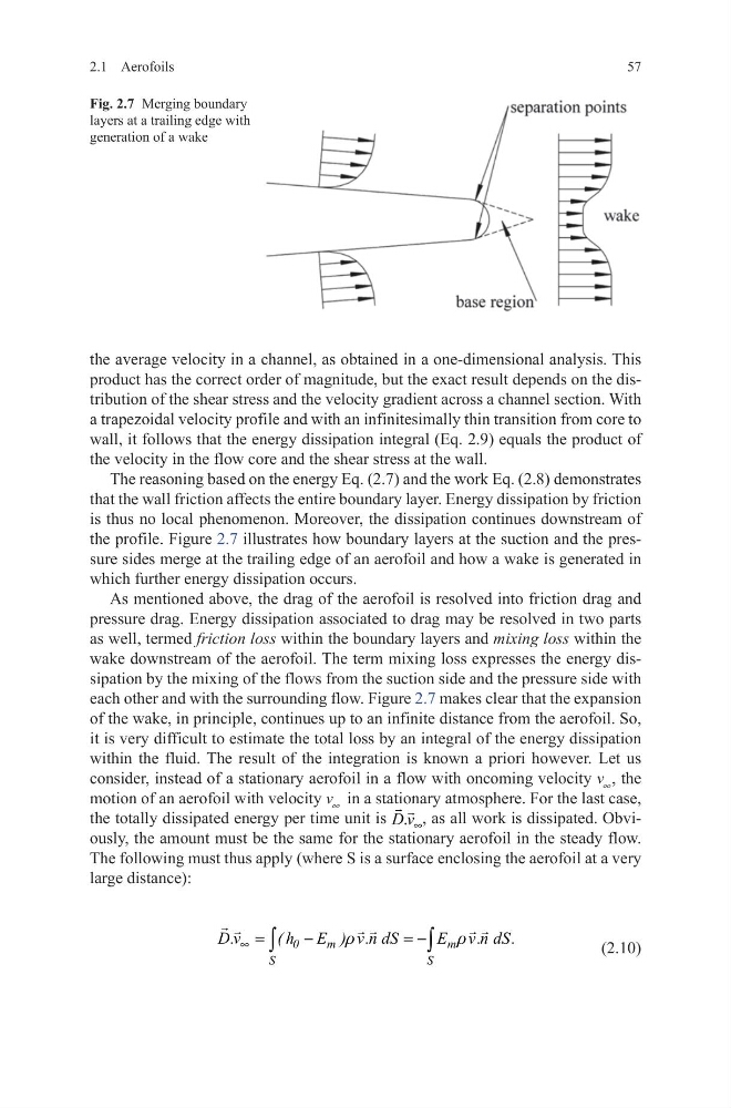
the profile. Figure 2.7 illustrates how boundary layers at the suction and the pressure sides merge at the trailing edge of an aerofoil and how a wake is generated in
which further energy dissipation occurs.
As mentioned above, the drag of the aerofoil is resolved into friction drag and
pressure drag. Energy dissipation associated to drag may be resolved in two parts
as well, termed friction loss within the boundary layers and mixing loss within the
wake downstream of the aerofoil. The term mixing loss expresses the energy dissipation by the mixing of the flows from the suction side and the pressure side with
each other and with the surrounding flow. Figure 2.7 makes clear that the expansion
of the wake, in principle, continues up to an infinite distance from the aerofoil. So,
it is very difficult to estimate the total loss by an integral of the energy dissipation
within the fluid. The result of the integration is known a priori however. Let us
consider, instead of a stationary aerofoil in a flow with oncoming velocity v ∞ , the
motion of an aerofoil with velocity v ∞ in a stationary atmosphere. For the last case,
the totally dissipated energy per time unit is .
D v ∞
, as all work is dissipated. Obviously, the amount must be the same for the stationary aerofoil in the steady flow.
The following must thus apply (where S is a surface enclosing the aerofoil at a very
large distance):
(2.10)
0
m
m
S
S
D.v
( h E ) v.n dS
E v.n dS .
r
r
∞ =
−
= −
∫
∫
Fig. 2.7 Merging boundary
layers at a trailing edge with
generation of a wake
2.1 Aerofoils
the average velocity in a channel, as obtained in a one-dimensional analysis. This
product has the correct order of magnitude, but the exact result depends on the distribution of the shear stress and the velocity gradient across a channel section. With
a trapezoidal velocity profile and with an infinitesimally thin transition from core to
wall, it follows that the energy dissipation integral (Eq. 2.9) equals the product of
the velocity in the flow core and the shear stress at the wall.
The reasoning based on the energy Eq. (2.7) and the work Eq. (2.8) demonstrates
that the wall friction affects the entire boundary layer. Energy dissipation by friction
is thus no local phenomenon. Moreover, the dissipation continues downstream of
the profile. Figure 2.7 illustrates how boundary layers at the suction and the pressure sides merge at the trailing edge of an aerofoil and how a wake is generated in
which further energy dissipation occurs.
As mentioned above, the drag of the aerofoil is resolved into friction drag and
pressure drag. Energy dissipation associated to drag may be resolved in two parts
as well, termed friction loss within the boundary layers and mixing loss within the
wake downstream of the aerofoil. The term mixing loss expresses the energy dissipation by the mixing of the flows from the suction side and the pressure side with
each other and with the surrounding flow. Figure 2.7 makes clear that the expansion
of the wake, in principle, continues up to an infinite distance from the aerofoil. So,
it is very difficult to estimate the total loss by an integral of the energy dissipation
within the fluid. The result of the integration is known a priori however. Let us
consider, instead of a stationary aerofoil in a flow with oncoming velocity v ∞ , the
motion of an aerofoil with velocity v ∞ in a stationary atmosphere. For the last case,
the totally dissipated energy per time unit is .
D v ∞
, as all work is dissipated. Obviously, the amount must be the same for the stationary aerofoil in the steady flow.
The following must thus apply (where S is a surface enclosing the aerofoil at a very
large distance):
(2.10)
0
m
m
S
S
D.v
( h E ) v.n dS
E v.n dS .
r
r
∞ =
−
= −
∫
∫
Fig. 2.7 Merging boundary
layers at a trailing edge with
generation of a wake