

365
10.3 Wind Turbine Performance Analysis
in the preceding section, but the expressions are more complicated and the solution
can only be found by means of numerical iteration. We do not discuss this here and
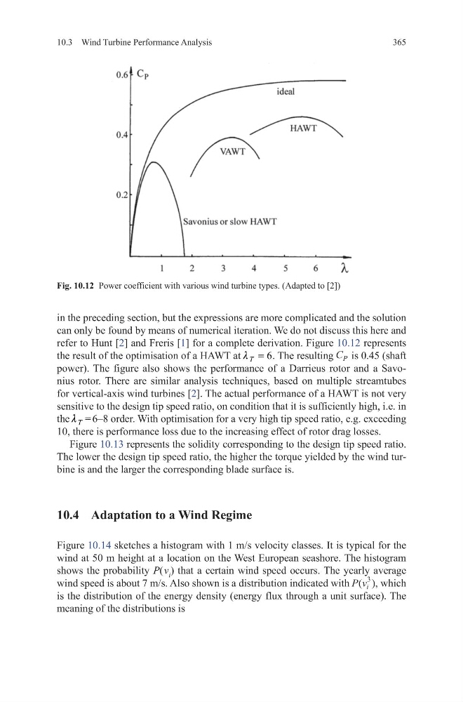
refer to Hunt [2] and Freris [1] for a complete derivation. Figure 10.12 represents
the result of the optimisation of a HAWT at
6
T
l = . The resulting C P is 0.45 (shaft
power). The figure also shows the performance of a Darrieus rotor and a Savonius rotor. There are similar analysis techniques, based on multiple streamtubes
for vertical-axis wind turbines [2]. The actual performance of a HAWT is not very
sensitive to the design tip speed ratio, on condition that it is sufficiently high, i.e. in
the T
l = 6–8 order. With optimisation for a very high tip speed ratio, e.g. exceeding
10, there is performance loss due to the increasing effect of rotor drag losses.
Figure 10.13 represents the solidity corresponding to the design tip speed ratio.
The lower the design tip speed ratio, the higher the torque yielded by the wind turbine is and the larger the corresponding blade surface is.
10.4 Adaptation to a Wind Regime
Figure 10.14 sketches a histogram with 1 m/s velocity classes. It is typical for the
wind at 50 m height at a location on the West European seashore. The histogram
shows the probability P( v i ) that a certain wind speed occurs. The yearly average
wind speed is about 7 m/s. Also shown is a distribution indicated with P v i
( ),
3
which
is the distribution of the energy density (energy flux through a unit surface). The
meaning of the distributions is
Fig. 10.12 Power coefficient with various wind turbine types. (Adapted to [2])
10.3 Wind Turbine Performance Analysis
in the preceding section, but the expressions are more complicated and the solution
can only be found by means of numerical iteration. We do not discuss this here and
refer to Hunt [2] and Freris [1] for a complete derivation. Figure 10.12 represents
the result of the optimisation of a HAWT at
6
T
l = . The resulting C P is 0.45 (shaft
power). The figure also shows the performance of a Darrieus rotor and a Savonius rotor. There are similar analysis techniques, based on multiple streamtubes
for vertical-axis wind turbines [2]. The actual performance of a HAWT is not very
sensitive to the design tip speed ratio, on condition that it is sufficiently high, i.e. in
the T
l = 6–8 order. With optimisation for a very high tip speed ratio, e.g. exceeding
10, there is performance loss due to the increasing effect of rotor drag losses.
Figure 10.13 represents the solidity corresponding to the design tip speed ratio.
The lower the design tip speed ratio, the higher the torque yielded by the wind turbine is and the larger the corresponding blade surface is.
10.4 Adaptation to a Wind Regime
Figure 10.14 sketches a histogram with 1 m/s velocity classes. It is typical for the
wind at 50 m height at a location on the West European seashore. The histogram
shows the probability P( v i ) that a certain wind speed occurs. The yearly average
wind speed is about 7 m/s. Also shown is a distribution indicated with P v i
( ),
3
which
is the distribution of the energy density (energy flux through a unit surface). The
meaning of the distributions is
Fig. 10.12 Power coefficient with various wind turbine types. (Adapted to [2])