

219
6.7 The Reaction Turbine
Ignoring the enthalpy increase by the divergence of the isobars, it applies that:
(6.18)
The negative root should be chosen in this case.
Iterative determination of the velocity components relative to v s , with given R s and l,
is quite simple. We take 1 72
°
=
a
as an example. We start iterations withv u
2
0
= ,
ss
h = 1, sr
h = 1. After a first calculation, we determine the flow angles and the loss
coefficients with Soderberg’s formula. Stator and rotor efficiency follow from
ss
h = 1/(1 + s
x ), sr
h = 1/(1 + r
x ). Table 6.2 represents the results for R s = 0, 0.25, 0.50
and 0.75.
Values in bold in Table 6.2 are those with optimum internal efficiency and with
a lower speed ratio corresponding to one and a half percentage points lower efficiency. Maximum efficiency is obtained with R s = 0.5. The reason is that the velocity
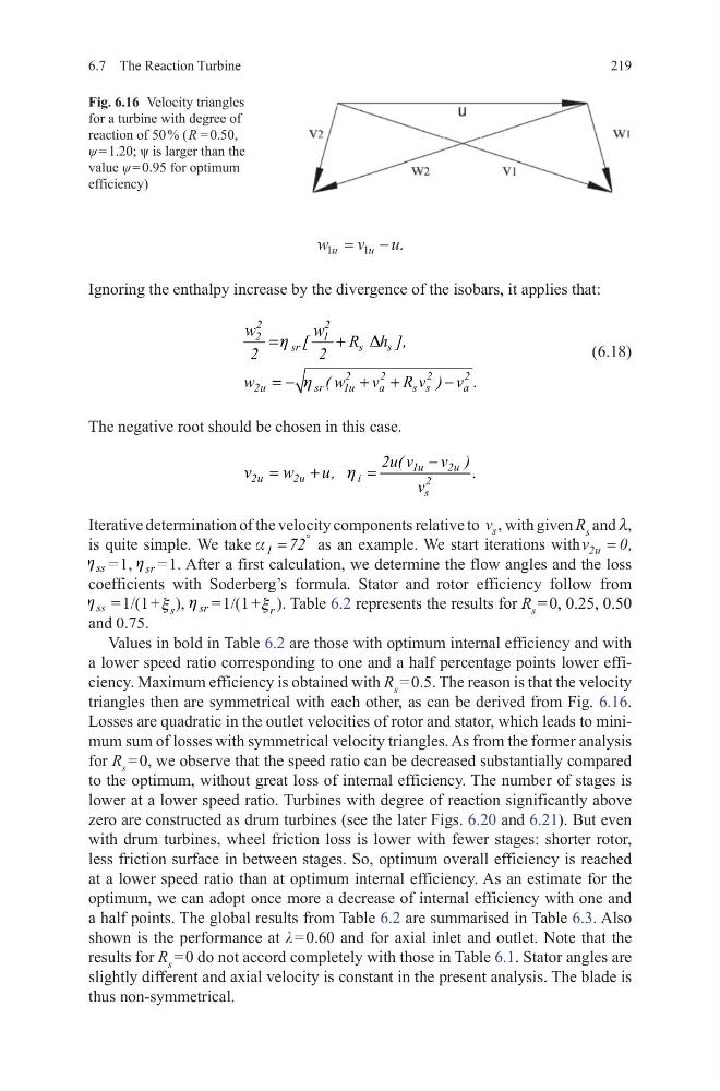
triangles then are symmetrical with each other, as can be derived from Fig. 6.16.
Losses are quadratic in the outlet velocities of rotor and stator, which leads to minimum sum of losses with symmetrical velocity triangles. As from the former analysis
for R s = 0, we observe that the speed ratio can be decreased substantially compared
to the optimum, without great loss of internal efficiency. The number of stages is
lower at a lower speed ratio. Turbines with degree of reaction significantly above
zero are constructed as drum turbines (see the later Figs. 6.20 and 6.21). But even
with drum turbines, wheel friction loss is lower with fewer stages: shorter rotor,
less friction surface in between stages. So, optimum overall efficiency is reached
at a lower speed ratio than at optimum internal efficiency. As an estimate for the
optimum, we can adopt once more a decrease of internal efficiency with one and
a half points. The global results from Table 6.2 are summarised in Table 6.3. Also
shown is the performance at λ = 0.60 and for axial inlet and outlet. Note that the
results for R s = 0 do not accord completely with those in Table 6.1. Stator angles are
slightly different and axial velocity is constant in the present analysis. The blade is
thus non-symmetrical.
w
v
u
u
u
1
1
=
− .
2
2
2
1
sr
s
s
2
2
2
2
2u
sr
1u
a
s s
a
w
w
[
R h ],
2
2
w
( w
v R
.
v ) v
h
D
h
=
+
= −
+ +
−
1u
2u
2u
2u
i
2
s
2u( v
v )
v
w
u,
.
v
−
=
+
=
h
Fig. 6.16 Velocity triangles
for a turbine with degree of
reaction of 50 % ( R = 0.50,
ψ = 1.20; ψ is larger than the
value ψ = 0.95 for optimum
efficiency)
6.7 The Reaction Turbine
Ignoring the enthalpy increase by the divergence of the isobars, it applies that:
(6.18)
The negative root should be chosen in this case.
Iterative determination of the velocity components relative to v s , with given R s and l,
is quite simple. We take 1 72
°
=
a
as an example. We start iterations withv u
2
0
= ,
ss
h = 1, sr
h = 1. After a first calculation, we determine the flow angles and the loss
coefficients with Soderberg’s formula. Stator and rotor efficiency follow from
ss
h = 1/(1 + s
x ), sr
h = 1/(1 + r
x ). Table 6.2 represents the results for R s = 0, 0.25, 0.50
and 0.75.
Values in bold in Table 6.2 are those with optimum internal efficiency and with
a lower speed ratio corresponding to one and a half percentage points lower efficiency. Maximum efficiency is obtained with R s = 0.5. The reason is that the velocity
triangles then are symmetrical with each other, as can be derived from Fig. 6.16.
Losses are quadratic in the outlet velocities of rotor and stator, which leads to minimum sum of losses with symmetrical velocity triangles. As from the former analysis
for R s = 0, we observe that the speed ratio can be decreased substantially compared
to the optimum, without great loss of internal efficiency. The number of stages is
lower at a lower speed ratio. Turbines with degree of reaction significantly above
zero are constructed as drum turbines (see the later Figs. 6.20 and 6.21). But even
with drum turbines, wheel friction loss is lower with fewer stages: shorter rotor,
less friction surface in between stages. So, optimum overall efficiency is reached
at a lower speed ratio than at optimum internal efficiency. As an estimate for the
optimum, we can adopt once more a decrease of internal efficiency with one and
a half points. The global results from Table 6.2 are summarised in Table 6.3. Also
shown is the performance at λ = 0.60 and for axial inlet and outlet. Note that the
results for R s = 0 do not accord completely with those in Table 6.1. Stator angles are
slightly different and axial velocity is constant in the present analysis. The blade is
thus non-symmetrical.
w
v
u
u
u
1
1
=
− .
2
2
2
1
sr
s
s
2
2
2
2
2u
sr
1u
a
s s
a
w
w
[
R h ],
2
2
w
( w
v R
.
v ) v
h
D
h
=
+
= −
+ +
−
1u
2u
2u
2u
i
2
s
2u( v
v )
v
w
u,
.
v
−
=
+
=
h
Fig. 6.16 Velocity triangles
for a turbine with degree of
reaction of 50 % ( R = 0.50,
ψ = 1.20; ψ is larger than the
value ψ = 0.95 for optimum
efficiency)