

158
4 Compressible Fluids
Thus, velocity of sound may be used as a measure for compressibility. Low velocity
of sound corresponds to high compressibility. From (4.12) and the ideal gas law, it
follows that
(4.13)
With an ideal gas, the velocity of sound only depends on temperature. For air
under atmospheric conditions ( γ = 1.4; R = 287 J/kgK; T = 288 K) it follows that
c = 340 m/s.
According to the compressibility definition, an incompressible fluid has an infinitely large elasticity modulus or an infinitely large speed of sound. No fluid is
strictly incompressible, however. A liquid is compressible, but much less than a gas.
For instance, water under atmospheric conditions ( p = 1 bar, T = 288 K) has a bulk
modulus E ≈ 2 10
9
Pa. The corresponding velocity of sound is c ≈ 1400 m/s, being
larger than with air, but with a ratio under one order of magnitude.
4.3 Compressibility Effect on the Velocity-Pressure
Relation
For a constant density fluid the relation between velocity and pressure follows from
the work equation or Bernoulli’s equation (4.2), by
(4.14)
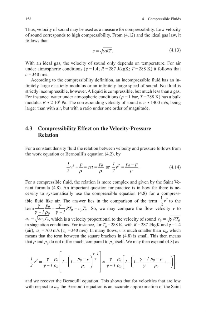
For a compressible fluid, the relation is more complex and given by the Saint Venant formula (4.8). An important question for practice is in how far there is necessity to systematically use the compressible equation (4.8) for a compressible fluid like air. The answer lies in the comparison of the term
1
2
2
v to the
term
0
0
p 0
0
p
RT c T
1
1
g
g
g
r
g
=
=
−
−
. So, we may compare the flow velocity v to
0
p 0
a
2c T
=
, which is a velocity proportional to the velocity of sound 0
0
c
RT
g
=
in stagnation conditions. For instance, for T 0 = 288 K, with R = 287 J/kgK and γ = 1.4
(air), a 0 = 760 m/s (c 0 = 340 m/s). In many flows, v is much smaller than a 0 , which
means that the term between the square brackets in (4.8) is small. This then means
that p and p 0 do not differ much, compared to p 0 itself. We may then expand (4.8) as
and we recover the Bernoulli equation. This shows that for velocities that are low
with respect to a 0 , the Bernoulli equation is an accurate approximation of the Saint
.
c
RT
g
=
or
.
2
2
0
0
p
p p
1
p
1
v
cst
v
2
2
r
r
r
−
+ =
=
=
1
2
0
0
0
0
0
0
0
0
p
p
p
p
p
p
1
1
v
1 1
1 1
... ,
2
1
p
1
p
g
g
g
g
g
g
r
g
r
g
−
−
−
−
=
− −
≈
− −
+
−
−
4 Compressible Fluids
Thus, velocity of sound may be used as a measure for compressibility. Low velocity
of sound corresponds to high compressibility. From (4.12) and the ideal gas law, it
follows that
(4.13)
With an ideal gas, the velocity of sound only depends on temperature. For air
under atmospheric conditions ( γ = 1.4; R = 287 J/kgK; T = 288 K) it follows that
c = 340 m/s.
According to the compressibility definition, an incompressible fluid has an infinitely large elasticity modulus or an infinitely large speed of sound. No fluid is
strictly incompressible, however. A liquid is compressible, but much less than a gas.
For instance, water under atmospheric conditions ( p = 1 bar, T = 288 K) has a bulk
modulus E ≈ 2 10
9
Pa. The corresponding velocity of sound is c ≈ 1400 m/s, being
larger than with air, but with a ratio under one order of magnitude.
4.3 Compressibility Effect on the Velocity-Pressure
Relation
For a constant density fluid the relation between velocity and pressure follows from
the work equation or Bernoulli’s equation (4.2), by
(4.14)
For a compressible fluid, the relation is more complex and given by the Saint Venant formula (4.8). An important question for practice is in how far there is necessity to systematically use the compressible equation (4.8) for a compressible fluid like air. The answer lies in the comparison of the term
1
2
2
v to the
term
0
0
p 0
0
p
RT c T
1
1
g
g
g
r
g
=
=
−
−
. So, we may compare the flow velocity v to
0
p 0
a
2c T
=
, which is a velocity proportional to the velocity of sound 0
0
c
RT
g
=
in stagnation conditions. For instance, for T 0 = 288 K, with R = 287 J/kgK and γ = 1.4
(air), a 0 = 760 m/s (c 0 = 340 m/s). In many flows, v is much smaller than a 0 , which
means that the term between the square brackets in (4.8) is small. This then means
that p and p 0 do not differ much, compared to p 0 itself. We may then expand (4.8) as
and we recover the Bernoulli equation. This shows that for velocities that are low
with respect to a 0 , the Bernoulli equation is an accurate approximation of the Saint
.
c
RT
g
=
or
.
2
2
0
0
p
p p
1
p
1
v
cst
v
2
2
r
r
r
−
+ =
=
=
1
2
0
0
0
0
0
0
0
0
p
p
p
p
p
p
1
1
v
1 1
1 1
... ,
2
1
p
1
p
g
g
g
g
g
g
r
g
r
g
−
−
−
−
=
− −
≈
− −
+
−
−