

366
Shalabh and S. S. Dhar
Residuals:
Next, we consider the outcome related to the residuals e = y ∼ ˆ
y. For example, the
fitted value ˆ
y 1 = ˆ
β 0 + x 11 ˆ
β 1 + x 12 ˆ
β 2 + x 13 ˆ
β 3 , which is obtained for given values of
x’s (x 11 = 18.3, x 12 = 29.1, x 13 = 52.0) as ˆ
y 1 = 22.2817 + 1.5817 × 18.3(x 11 ) +
0.5504 × 29.1(x 12 ) + 1.0963 × 52.0(x 13 ) = 124.251 and y 1 = 122.0, so residual
corresponding to the first set of observation is e 1 = y 1 − ˆ
y 1 = −2.251. Other values
of residuals can be found similarly. The following outcome
Residuals:
Min
1Q
Median
3Q
Max
-1.09906 -0.87756 -0.07462 0.70157 1.39258
provides the information on the distribution of the values of residuals in terms of their
minimum value (Min=-1.09906), maximum value (Max=1.39258), first quartile (1Q=-0.87756), second quartile (Median=-0.07462) and third quartile
(3Q=0.70157).
Analysis of variance:
The
outcome
F-statistic: 145.8 on 3 and 6 DF, p-value:
5.395e-06 gives the value of the F-Statistics F =
M S reg
M S err or
related to the analysis
of variance. It tests H 0 : β 1 = β 2 = β 3 = 0 against the alternative hypothesis
H 1 : β j = 0 for at least one j = 1, 2, 3 with k = 3 and n − k − 1 = 6 degrees of
freedom with corresponding p-value = 5.395 × 10
−06 , which is less than the level
of significance α = 0.05. This indicates that H 0 : β 1 = β 2 = β 3 = 0 is rejected.
Confidence interval:
The 100(1 − α)% confidence interval of β j ( j = 0, 1, 2, . . . , k) is given by ˆ
β j −
t α
2 ,n−k−1
ˆ
σ 2 C j j ≤ β j ≤ ˆ
β j + t α
2 ,n−k−1
ˆ
σ 2 C j j . The 95% confidence intervals
with α = 0.05 for intercept term and regression coefficients are obtained by the R
command confint() as follows:
> confint(lm(rain~ windspeed + precipitation + relhum), level = 0.95)
2.5 %
97.5 %
(Intercept)
6.7535814 37.8097335
windspeed
0.9879101 2.0495022
precipitation 0.2439594 0.8567413
relhum
0.9500208 1.2426673
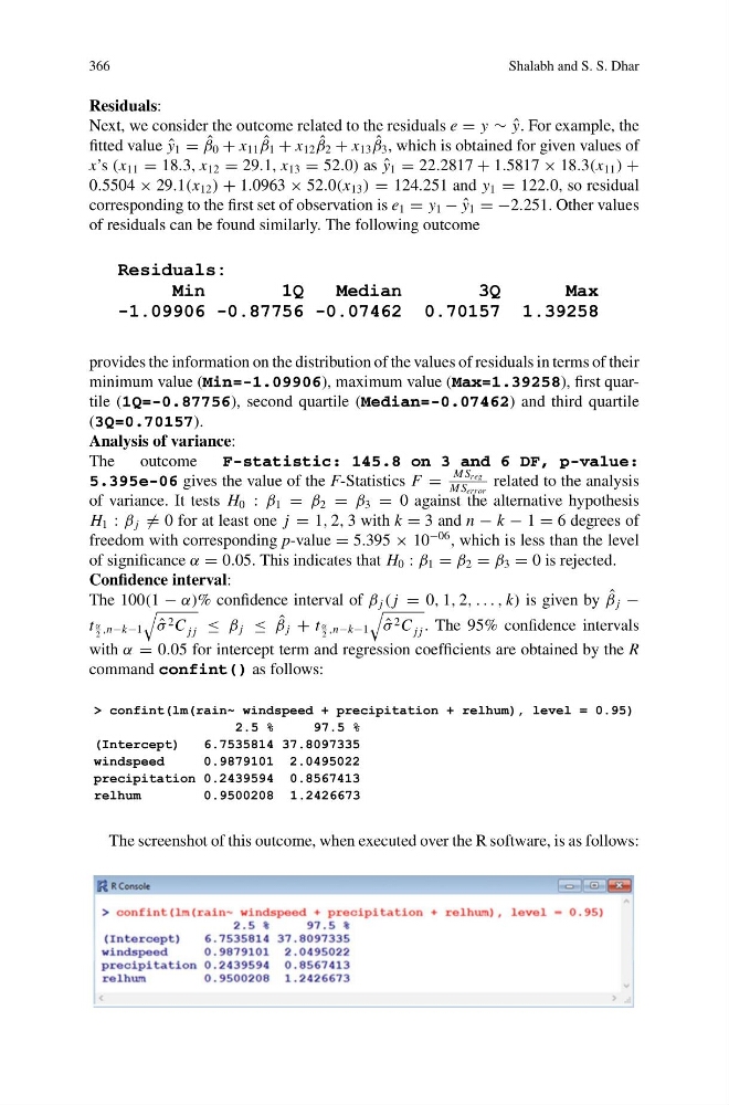
The screenshot of this outcome, when executed over the R software, is as follows:
Shalabh and S. S. Dhar
Residuals:
Next, we consider the outcome related to the residuals e = y ∼ ˆ
y. For example, the
fitted value ˆ
y 1 = ˆ
β 0 + x 11 ˆ
β 1 + x 12 ˆ
β 2 + x 13 ˆ
β 3 , which is obtained for given values of
x’s (x 11 = 18.3, x 12 = 29.1, x 13 = 52.0) as ˆ
y 1 = 22.2817 + 1.5817 × 18.3(x 11 ) +
0.5504 × 29.1(x 12 ) + 1.0963 × 52.0(x 13 ) = 124.251 and y 1 = 122.0, so residual
corresponding to the first set of observation is e 1 = y 1 − ˆ
y 1 = −2.251. Other values
of residuals can be found similarly. The following outcome
Residuals:
Min
1Q
Median
3Q
Max
-1.09906 -0.87756 -0.07462 0.70157 1.39258
provides the information on the distribution of the values of residuals in terms of their
minimum value (Min=-1.09906), maximum value (Max=1.39258), first quartile (1Q=-0.87756), second quartile (Median=-0.07462) and third quartile
(3Q=0.70157).
Analysis of variance:
The
outcome
F-statistic: 145.8 on 3 and 6 DF, p-value:
5.395e-06 gives the value of the F-Statistics F =
M S reg
M S err or
related to the analysis
of variance. It tests H 0 : β 1 = β 2 = β 3 = 0 against the alternative hypothesis
H 1 : β j = 0 for at least one j = 1, 2, 3 with k = 3 and n − k − 1 = 6 degrees of
freedom with corresponding p-value = 5.395 × 10
−06 , which is less than the level
of significance α = 0.05. This indicates that H 0 : β 1 = β 2 = β 3 = 0 is rejected.
Confidence interval:
The 100(1 − α)% confidence interval of β j ( j = 0, 1, 2, . . . , k) is given by ˆ
β j −
t α
2 ,n−k−1
ˆ
σ 2 C j j ≤ β j ≤ ˆ
β j + t α
2 ,n−k−1
ˆ
σ 2 C j j . The 95% confidence intervals
with α = 0.05 for intercept term and regression coefficients are obtained by the R
command confint() as follows:
> confint(lm(rain~ windspeed + precipitation + relhum), level = 0.95)
2.5 %
97.5 %
(Intercept)
6.7535814 37.8097335
windspeed
0.9879101 2.0495022
precipitation 0.2439594 0.8567413
relhum
0.9500208 1.2426673
The screenshot of this outcome, when executed over the R software, is as follows: