

15.2 Experimental Set-Up
Appropriate equipment and model setup are necessary in order to capture kinematic motion. Digital image correlation (DIC)
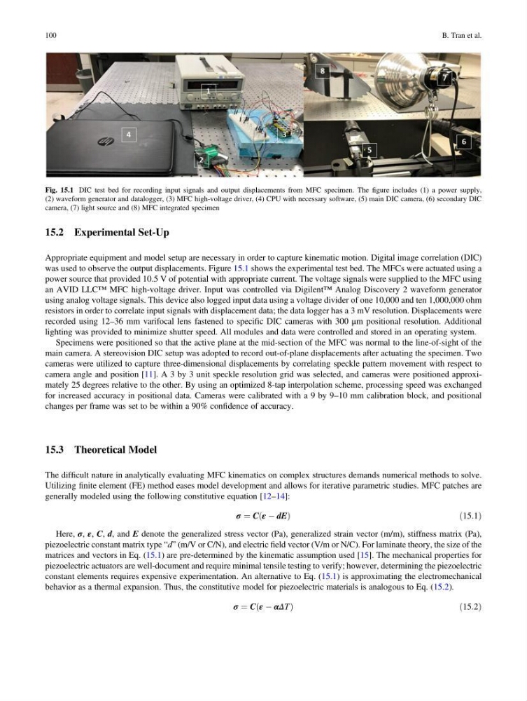
was used to observe the output displacements. Figure 15.1 shows the experimental test bed. The MFCs were actuated using a
power source that provided 10.5 V of potential with appropriate current. The voltage signals were supplied to the MFC using
an AVID LLC™ MFC high-voltage driver. Input was controlled via Digilent™ Analog Discovery 2 waveform generator
using analog voltage signals. This device also logged input data using a voltage divider of one 10,000 and ten 1,000,000 ohm
resistors in order to correlate input signals with displacement data; the data logger has a 3 mV resolution. Displacements were
recorded using 12–36 mm varifocal lens fastened to specific DIC cameras with 300 μm positional resolution. Additional
lighting was provided to minimize shutter speed. All modules and data were controlled and stored in an operating system.
Specimens were positioned so that the active plane at the mid-section of the MFC was normal to the line-of-sight of the
main camera. A stereovision DIC setup was adopted to record out-of-plane displacements after actuating the specimen. Two
cameras were utilized to capture three-dimensional displacements by correlating speckle pattern movement with respect to
camera angle and position [11]. A 3 by 3 unit speckle resolution grid was selected, and cameras were positioned approximately 25 degrees relative to the other. By using an optimized 8-tap interpolation scheme, processing speed was exchanged
for increased accuracy in positional data. Cameras were calibrated with a 9 by 9–10 mm calibration block, and positional
changes per frame was set to be within a 90% confidence of accuracy.
15.3 Theoretical Model
The difficult nature in analytically evaluating MFC kinematics on complex structures demands numerical methods to solve.
Utilizing finite element (FE) method eases model development and allows for iterative parametric studies. MFC patches are
generally modeled using the following constitutive equation [12–14]:
σ ¼ C ε À dE
ð
Þ
ð15:1Þ
Here, σ, ε, C, d, and E denote the generalized stress vector (Pa), generalized strain vector (m/m), stiffness matrix (Pa),
piezoelectric constant matrix type “d” (m/V or C/N), and electric field vector (V/m or N/C). For laminate theory, the size of the
matrices and vectors in Eq. (15.1) are pre-determined by the kinematic assumption used [15]. The mechanical properties for
piezoelectric actuators are well-document and require minimal tensile testing to verify; however, determining the piezoelectric
constant elements requires expensive experimentation. An alternative to Eq. (15.1) is approximating the electromechanical
behavior as a thermal expansion. Thus, the constitutive model for piezoelectric materials is analogous to Eq. (15.2).
σ ¼ C ε À αΔT
ð
Þ
ð 15:2Þ
Fig. 15.1 DIC test bed for recording input signals and output displacements from MFC specimen. The figure includes (1) a power supply,
(2) waveform generator and datalogger, (3) MFC high-voltage driver, (4) CPU with necessary software, (5) main DIC camera, (6) secondary DIC
camera, (7) light source and (8) MFC integrated specimen
100
B. Tran et al.
Appropriate equipment and model setup are necessary in order to capture kinematic motion. Digital image correlation (DIC)
was used to observe the output displacements. Figure 15.1 shows the experimental test bed. The MFCs were actuated using a
power source that provided 10.5 V of potential with appropriate current. The voltage signals were supplied to the MFC using
an AVID LLC™ MFC high-voltage driver. Input was controlled via Digilent™ Analog Discovery 2 waveform generator
using analog voltage signals. This device also logged input data using a voltage divider of one 10,000 and ten 1,000,000 ohm
resistors in order to correlate input signals with displacement data; the data logger has a 3 mV resolution. Displacements were
recorded using 12–36 mm varifocal lens fastened to specific DIC cameras with 300 μm positional resolution. Additional
lighting was provided to minimize shutter speed. All modules and data were controlled and stored in an operating system.
Specimens were positioned so that the active plane at the mid-section of the MFC was normal to the line-of-sight of the
main camera. A stereovision DIC setup was adopted to record out-of-plane displacements after actuating the specimen. Two
cameras were utilized to capture three-dimensional displacements by correlating speckle pattern movement with respect to
camera angle and position [11]. A 3 by 3 unit speckle resolution grid was selected, and cameras were positioned approximately 25 degrees relative to the other. By using an optimized 8-tap interpolation scheme, processing speed was exchanged
for increased accuracy in positional data. Cameras were calibrated with a 9 by 9–10 mm calibration block, and positional
changes per frame was set to be within a 90% confidence of accuracy.
15.3 Theoretical Model
The difficult nature in analytically evaluating MFC kinematics on complex structures demands numerical methods to solve.
Utilizing finite element (FE) method eases model development and allows for iterative parametric studies. MFC patches are
generally modeled using the following constitutive equation [12–14]:
σ ¼ C ε À dE
ð
Þ
ð15:1Þ
Here, σ, ε, C, d, and E denote the generalized stress vector (Pa), generalized strain vector (m/m), stiffness matrix (Pa),
piezoelectric constant matrix type “d” (m/V or C/N), and electric field vector (V/m or N/C). For laminate theory, the size of the
matrices and vectors in Eq. (15.1) are pre-determined by the kinematic assumption used [15]. The mechanical properties for
piezoelectric actuators are well-document and require minimal tensile testing to verify; however, determining the piezoelectric
constant elements requires expensive experimentation. An alternative to Eq. (15.1) is approximating the electromechanical
behavior as a thermal expansion. Thus, the constitutive model for piezoelectric materials is analogous to Eq. (15.2).
σ ¼ C ε À αΔT
ð
Þ
ð 15:2Þ
Fig. 15.1 DIC test bed for recording input signals and output displacements from MFC specimen. The figure includes (1) a power supply,
(2) waveform generator and datalogger, (3) MFC high-voltage driver, (4) CPU with necessary software, (5) main DIC camera, (6) secondary DIC
camera, (7) light source and (8) MFC integrated specimen
100
B. Tran et al.