

2.3 SHPB Test
35
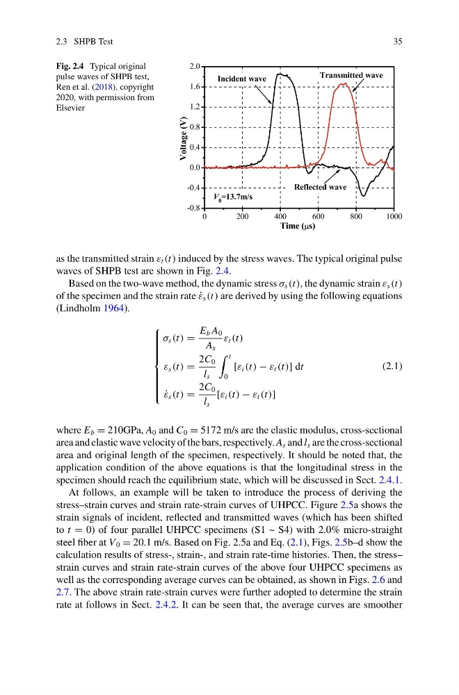
Fig. 2.4 Typical original
pulse waves of SHPB test,
Ren et al. (2018), copyright
2020, with permission from
Elsevier
as the transmitted strain ε t (t) induced by the stress waves. The typical original pulse
waves of SHPB test are shown in Fig. 2.4.
Based on the two-wave method, the dynamic stress σ s (t), the dynamic strain ε s (t)
of the specimen and the strain rate ˙
ε s (t) are derived by using the following equations
(Lindholm 1964).
⎧
⎪ ⎪ ⎪ ⎪ ⎪ ⎪ ⎨
⎪ ⎪ ⎪ ⎪ ⎪ ⎪ ⎩
σ s (t) =
E b A 0
A s
ε t (t)
ε s (t) =
2C 0
l s
t
0
[ε i (t) − ε t (t)] dt
˙
ε s (t) =
2C 0
l s
[ε i (t) − ε t (t)]
(2.1)
where E b = 210GPa, A 0 and C 0 = 5172 m/s are the elastic modulus, cross-sectional
area and elastic wave velocity of the bars, respectively. A s and l s are the cross-sectional
area and original length of the specimen, respectively. It should be noted that, the
application condition of the above equations is that the longitudinal stress in the
specimen should reach the equilibrium state, which will be discussed in Sect. 2.4.1.
At follows, an example will be taken to introduce the process of deriving the
stress–strain curves and strain rate-strain curves of UHPCC. Figure 2.5a shows the
strain signals of incident, reflected and transmitted waves (which has been shifted
to t = 0) of four parallel UHPCC specimens (S1 ~ S4) with 2.0% micro-straight
steel fiber at V 0 = 20.1 m/s. Based on Fig. 2.5a and Eq. (2.1), Figs. 2.5b–d show the
calculation results of stress-, strain-, and strain rate-time histories. Then, the stress–
strain curves and strain rate-strain curves of the above four UHPCC specimens as
well as the corresponding average curves can be obtained, as shown in Figs. 2.6 and
2.7. The above strain rate-strain curves were further adopted to determine the strain
rate at follows in Sect. 2.4.2. It can be seen that, the average curves are smoother
35
Fig. 2.4 Typical original
pulse waves of SHPB test,
Ren et al. (2018), copyright
2020, with permission from
Elsevier
as the transmitted strain ε t (t) induced by the stress waves. The typical original pulse
waves of SHPB test are shown in Fig. 2.4.
Based on the two-wave method, the dynamic stress σ s (t), the dynamic strain ε s (t)
of the specimen and the strain rate ˙
ε s (t) are derived by using the following equations
(Lindholm 1964).
⎧
⎪ ⎪ ⎪ ⎪ ⎪ ⎪ ⎨
⎪ ⎪ ⎪ ⎪ ⎪ ⎪ ⎩
σ s (t) =
E b A 0
A s
ε t (t)
ε s (t) =
2C 0
l s
t
0
[ε i (t) − ε t (t)] dt
˙
ε s (t) =
2C 0
l s
[ε i (t) − ε t (t)]
(2.1)
where E b = 210GPa, A 0 and C 0 = 5172 m/s are the elastic modulus, cross-sectional
area and elastic wave velocity of the bars, respectively. A s and l s are the cross-sectional
area and original length of the specimen, respectively. It should be noted that, the
application condition of the above equations is that the longitudinal stress in the
specimen should reach the equilibrium state, which will be discussed in Sect. 2.4.1.
At follows, an example will be taken to introduce the process of deriving the
stress–strain curves and strain rate-strain curves of UHPCC. Figure 2.5a shows the
strain signals of incident, reflected and transmitted waves (which has been shifted
to t = 0) of four parallel UHPCC specimens (S1 ~ S4) with 2.0% micro-straight
steel fiber at V 0 = 20.1 m/s. Based on Fig. 2.5a and Eq. (2.1), Figs. 2.5b–d show the
calculation results of stress-, strain-, and strain rate-time histories. Then, the stress–
strain curves and strain rate-strain curves of the above four UHPCC specimens as
well as the corresponding average curves can be obtained, as shown in Figs. 2.6 and
2.7. The above strain rate-strain curves were further adopted to determine the strain
rate at follows in Sect. 2.4.2. It can be seen that, the average curves are smoother