

11.3 Analytical Methods for Predicting the Dynamic Responses …
387
Eq. (11.15) and the corresponding initial conditions are given in Eq. (11.12).
K LM M ¨
z(t) + k M z(t) = 0
(11.15)
When t e < t ≤ t m , t m is the time instant when the deformation of the system
reaches the ultimate state, the system is in the plastic stage and its differential motion
equation is given in Eq. (11.16), and the corresponding initial conditions are given
in Eq. (11.17).
K LM M ¨
z(t) + R u = 0
(11.16)
z(t e ) = z e , v(t e ) = ˙
z(t e ) =
dz
dt
t=t e
(11.17)
When t > t m , the system is in the resilient stage and the corresponding differential
motion equation is given in Eq. (11.18). In this stage, the damping should be considered to make the system stabilized and stopped. The corresponding initial conditions
are given in Eq. (11.19).
K LM M ¨
z(t) + c˙ z(t) + k M
z(t) − z p
= 0
(11.18)
z(t m ) = z m , v(t m ) = ˙
z(t m ) = 0
(11.19)
where z m can be calculated by Eq. (11.16) of the system during plastic period.
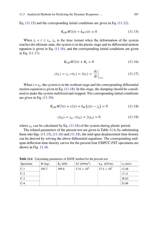
The related parameters of the present test are given in Table 11.6, by substituting
them into Eqs. (11.15), (11.16) and (11.18), the mid-span displacement time-history
can be derived by solving the above differential equations. The corresponding midspan deflection time-history curves for the present four UHPCC-FST specimens are
shown in Fig. 11.16.
Table 11.6 Calculating parameters of SDOF method for the present test
Specimen
M (kg)
R u (kN)
EJ (kN•m 2 )
k M (kN/m)
v 0 (m/s)
C-1
185.7
399.8
5.34 × 10 3
37.4 × 10 3
13.46
C-2
17.11
C-3
28.63
C-4
33.46
387
Eq. (11.15) and the corresponding initial conditions are given in Eq. (11.12).
K LM M ¨
z(t) + k M z(t) = 0
(11.15)
When t e < t ≤ t m , t m is the time instant when the deformation of the system
reaches the ultimate state, the system is in the plastic stage and its differential motion
equation is given in Eq. (11.16), and the corresponding initial conditions are given
in Eq. (11.17).
K LM M ¨
z(t) + R u = 0
(11.16)
z(t e ) = z e , v(t e ) = ˙
z(t e ) =
dz
dt
t=t e
(11.17)
When t > t m , the system is in the resilient stage and the corresponding differential
motion equation is given in Eq. (11.18). In this stage, the damping should be considered to make the system stabilized and stopped. The corresponding initial conditions
are given in Eq. (11.19).
K LM M ¨
z(t) + c˙ z(t) + k M
z(t) − z p
= 0
(11.18)
z(t m ) = z m , v(t m ) = ˙
z(t m ) = 0
(11.19)
where z m can be calculated by Eq. (11.16) of the system during plastic period.
The related parameters of the present test are given in Table 11.6, by substituting
them into Eqs. (11.15), (11.16) and (11.18), the mid-span displacement time-history
can be derived by solving the above differential equations. The corresponding midspan deflection time-history curves for the present four UHPCC-FST specimens are
shown in Fig. 11.16.
Table 11.6 Calculating parameters of SDOF method for the present test
Specimen
M (kg)
R u (kN)
EJ (kN•m 2 )
k M (kN/m)
v 0 (m/s)
C-1
185.7
399.8
5.34 × 10 3
37.4 × 10 3
13.46
C-2
17.11
C-3
28.63
C-4
33.46