

382
11 Experimental and Numerical Study of UHPCC-FST Columns …
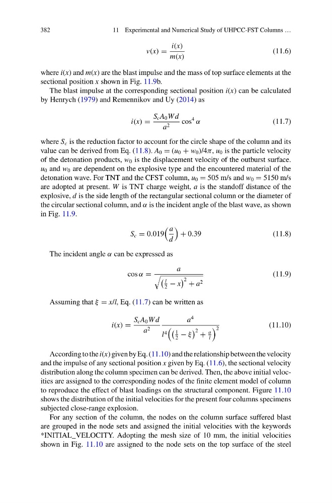
v(x) =
i(x)
m(x)
(11.6)
where i(x) and m(x) are the blast impulse and the mass of top surface elements at the
sectional position x shown in Fig. 11.9b.
The blast impulse at the corresponding sectional position i(x) can be calculated
by Henrych (1979) and Remennikov and Uy (2014) as
i(x) =
S c A 0 W d
a 2
cos
4
α
(11.7)
where S c is the reduction factor to account for the circle shape of the column and its
value can be derived from Eq. (11.8). A 0 = (u 0 + w 0 )/4π, u 0 is the particle velocity
of the detonation products, w 0 is the displacement velocity of the outburst surface.
u 0 and w 0 are dependent on the explosive type and the encountered material of the
detonation wave. For TNT and the CFST column, u 0 = 505 m/s and w 0 = 5150 m/s
are adopted at present. W is TNT charge weight, a is the standoff distance of the
explosive, d is the side length of the rectangular sectional column or the diameter of
the circular sectional column, and α is the incident angle of the blast wave, as shown
in Fig. 11.9.
S c = 0.019
a
d
+ 0.39
(11.8)
The incident angle α can be expressed as
cos α =
a
l
2
− x
2 + a 2
(11.9)
Assuming that ξ = x/l, Eq. (11.7) can be written as
i(x) =
S c A 0 W d
a 2
a
4
l 4
1
2
− ξ
2 +
a
l
2
(11.10)
According to the i(x) given by Eq. (11.10) and the relationship between the velocity
and the impulse of any sectional position x given by Eq. (11.6), the sectional velocity
distribution along the column specimen can be derived. Then, the above initial velocities are assigned to the corresponding nodes of the finite element model of column
to reproduce the effect of blast loadings on the structural component. Figure 11.10
shows the distribution of the initial velocities for the present four columns specimens
subjected close-range explosion.
For any section of the column, the nodes on the column surface suffered blast
are grouped in the node sets and assigned the initial velocities with the keywords
*INITIAL_VELOCITY. Adopting the mesh size of 10 mm, the initial velocities
shown in Fig. 11.10 are assigned to the node sets on the top surface of the steel
11 Experimental and Numerical Study of UHPCC-FST Columns …
v(x) =
i(x)
m(x)
(11.6)
where i(x) and m(x) are the blast impulse and the mass of top surface elements at the
sectional position x shown in Fig. 11.9b.
The blast impulse at the corresponding sectional position i(x) can be calculated
by Henrych (1979) and Remennikov and Uy (2014) as
i(x) =
S c A 0 W d
a 2
cos
4
α
(11.7)
where S c is the reduction factor to account for the circle shape of the column and its
value can be derived from Eq. (11.8). A 0 = (u 0 + w 0 )/4π, u 0 is the particle velocity
of the detonation products, w 0 is the displacement velocity of the outburst surface.
u 0 and w 0 are dependent on the explosive type and the encountered material of the
detonation wave. For TNT and the CFST column, u 0 = 505 m/s and w 0 = 5150 m/s
are adopted at present. W is TNT charge weight, a is the standoff distance of the
explosive, d is the side length of the rectangular sectional column or the diameter of
the circular sectional column, and α is the incident angle of the blast wave, as shown
in Fig. 11.9.
S c = 0.019
a
d
+ 0.39
(11.8)
The incident angle α can be expressed as
cos α =
a
l
2
− x
2 + a 2
(11.9)
Assuming that ξ = x/l, Eq. (11.7) can be written as
i(x) =
S c A 0 W d
a 2
a
4
l 4
1
2
− ξ
2 +
a
l
2
(11.10)
According to the i(x) given by Eq. (11.10) and the relationship between the velocity
and the impulse of any sectional position x given by Eq. (11.6), the sectional velocity
distribution along the column specimen can be derived. Then, the above initial velocities are assigned to the corresponding nodes of the finite element model of column
to reproduce the effect of blast loadings on the structural component. Figure 11.10
shows the distribution of the initial velocities for the present four columns specimens
subjected close-range explosion.
For any section of the column, the nodes on the column surface suffered blast
are grouped in the node sets and assigned the initial velocities with the keywords
*INITIAL_VELOCITY. Adopting the mesh size of 10 mm, the initial velocities
shown in Fig. 11.10 are assigned to the node sets on the top surface of the steel