

9.7 Size-Dependent Euler-Bernoulli Beams with Topologically Optimized Microstructure 377
9.7.2 Mathematical Background
9.7.2.1 Topological Optimization
Consider a 2D elastic beam area , bounded by the closed surface = 1 ∪ 2 ∪
3 and subjected to a plane stress state. We assume that the material of beams is
linearly elastic and isotropic and that it is subjected to the temperature field T (x), x =
{x 1 , x 3 }.
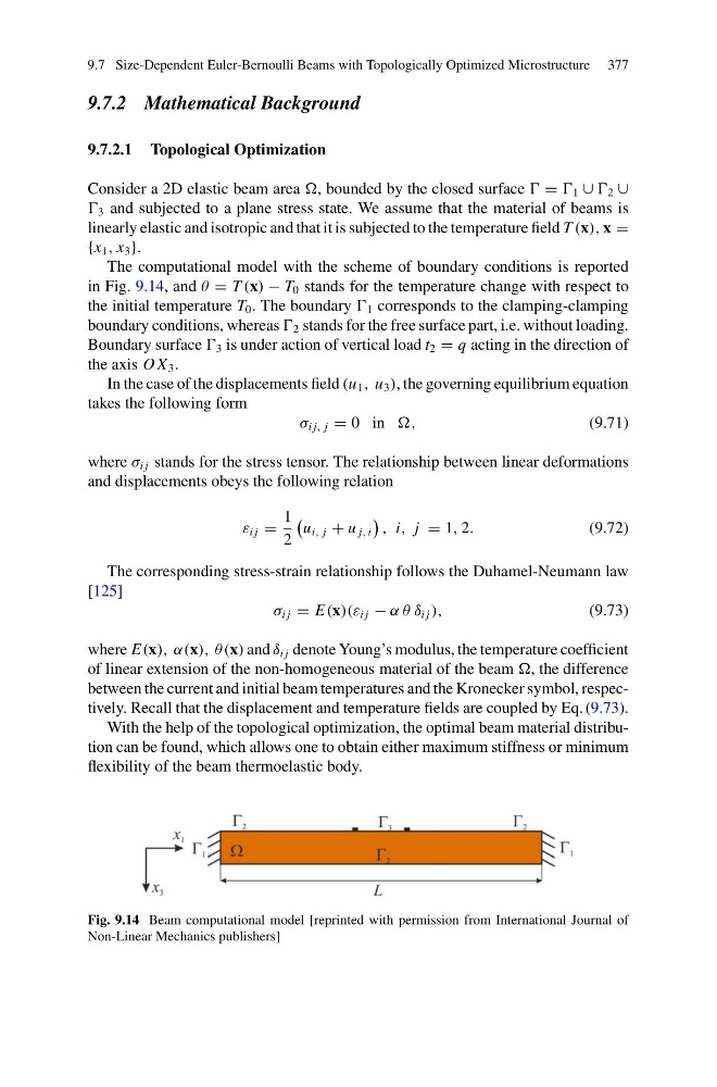
The computational model with the scheme of boundary conditions is reported
in Fig. 9.14, and θ = T (x) − T 0 stands for the temperature change with respect to
the initial temperature T 0 . The boundary 1 corresponds to the clamping-clamping
boundary conditions, whereas 2 stands for the free surface part, i.e. without loading.
Boundary surface 3 is under action of vertical load t 2 = q acting in the direction of
the axis O X 3 .
In the case of the displacements field (u 1 , u 3 ), the governing equilibrium equation
takes the following form
σ i j, j = 0 in ,
(9.71)
where σ i j stands for the stress tensor. The relationship between linear deformations
and displacements obeys the following relation
ε i j =
1
2
u i, j + u j, i
, i, j = 1, 2.
(9.72)
The corresponding stress-strain relationship follows the Duhamel-Neumann law
[125]
σ i j = E(x)(ε i j − α θ δ i j ),
(9.73)
where E(x), α(x), θ (x) and δ i j denote Young’s modulus, the temperature coefficient
of linear extension of the non-homogeneous material of the beam , the difference
between the current and initial beam temperatures and the Kronecker symbol, respectively. Recall that the displacement and temperature fields are coupled by Eq. (9.73).
With the help of the topological optimization, the optimal beam material distribution can be found, which allows one to obtain either maximum stiffness or minimum
flexibility of the beam thermoelastic body.
Fig. 9.14 Beam computational model [reprinted with permission from International Journal of
Non-Linear Mechanics publishers]
9.7.2 Mathematical Background
9.7.2.1 Topological Optimization
Consider a 2D elastic beam area , bounded by the closed surface = 1 ∪ 2 ∪
3 and subjected to a plane stress state. We assume that the material of beams is
linearly elastic and isotropic and that it is subjected to the temperature field T (x), x =
{x 1 , x 3 }.
The computational model with the scheme of boundary conditions is reported
in Fig. 9.14, and θ = T (x) − T 0 stands for the temperature change with respect to
the initial temperature T 0 . The boundary 1 corresponds to the clamping-clamping
boundary conditions, whereas 2 stands for the free surface part, i.e. without loading.
Boundary surface 3 is under action of vertical load t 2 = q acting in the direction of
the axis O X 3 .
In the case of the displacements field (u 1 , u 3 ), the governing equilibrium equation
takes the following form
σ i j, j = 0 in ,
(9.71)
where σ i j stands for the stress tensor. The relationship between linear deformations
and displacements obeys the following relation
ε i j =
1
2
u i, j + u j, i
, i, j = 1, 2.
(9.72)
The corresponding stress-strain relationship follows the Duhamel-Neumann law
[125]
σ i j = E(x)(ε i j − α θ δ i j ),
(9.73)
where E(x), α(x), θ (x) and δ i j denote Young’s modulus, the temperature coefficient
of linear extension of the non-homogeneous material of the beam , the difference
between the current and initial beam temperatures and the Kronecker symbol, respectively. Recall that the displacement and temperature fields are coupled by Eq. (9.73).
With the help of the topological optimization, the optimal beam material distribution can be found, which allows one to obtain either maximum stiffness or minimum
flexibility of the beam thermoelastic body.
Fig. 9.14 Beam computational model [reprinted with permission from International Journal of
Non-Linear Mechanics publishers]