

364
9 Topologic Optimization of Vibrations of Size-Dependent Beams
χ
i j
1 = 0 and on y 2 = 0, y 2 = Y 2 , χ
i j
2 = 0 (Fig. 9.8b); in the case of load i j = 12 (or
21) on y 1 = 0, y 1 = Y 1 , χ
12
2 = 0 and on y 2 = 0, y 2 = Y 2 , χ
12
1 = 0 (Fig. 9.8c).
9.6.3 Determination of the Effective Heat Transfer
Coefficient
To calculate the effective heat transfer coefficient of an elementary periodic cell, the
homogenization method is applied, and the associated homogenized terms can be
obtained from heat transfer equations. According to references [45, 46, 68, 112], the
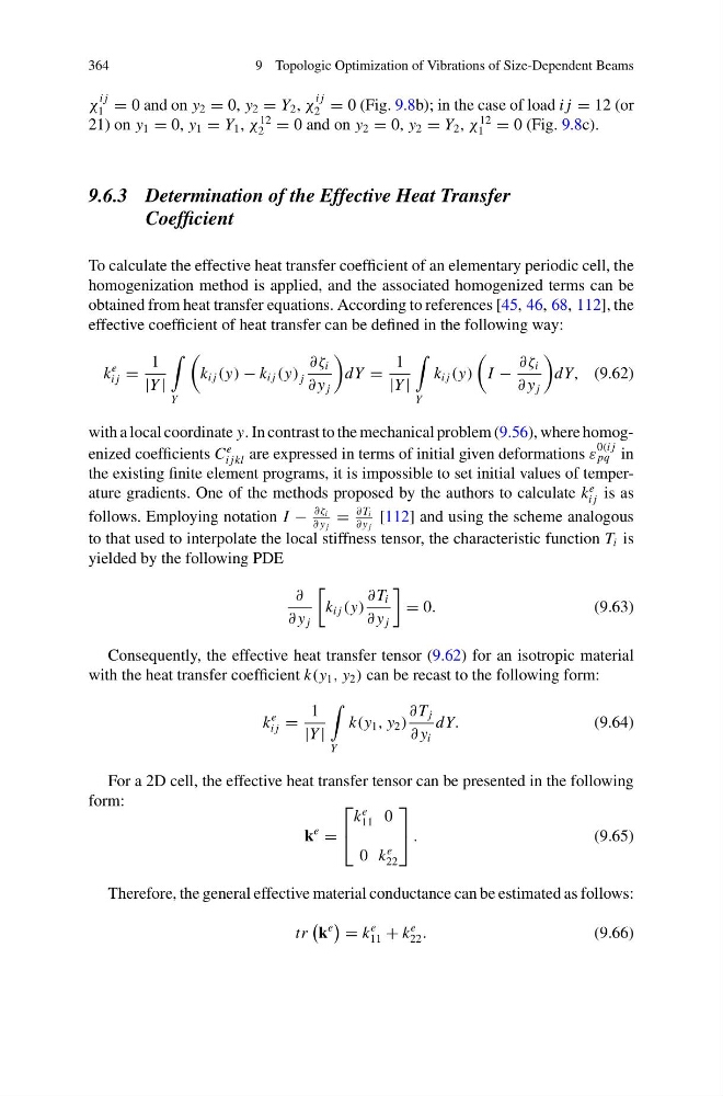
effective coefficient of heat transfer can be defined in the following way:
k
e
i j =
1
|Y |
Y
k i j (y) − k i j (y) j
∂ζ i
∂ y j
dY =
1
|Y |
Y
k i j (y)
I −
∂ζ i
∂ y j
dY, (9.62)
with a local coordinate y. In contrast to the mechanical problem (9.56), where homogenized coefficients C
e
i jkl are expressed in terms of initial given deformations ε
0(i j
pq in
the existing finite element programs, it is impossible to set initial values of temperature gradients. One of the methods proposed by the authors to calculate k
e
i j is as
follows. Employing notation I −
∂ζ i
∂ y j
=
∂ T i
∂ y j
[112] and using the scheme analogous
to that used to interpolate the local stiffness tensor, the characteristic function T i is
yielded by the following PDE
∂
∂ y j
k i j (y)
∂ T i
∂ y j
= 0.
(9.63)
Consequently, the effective heat transfer tensor (9.62) for an isotropic material
with the heat transfer coefficient k(y 1 , y 2 ) can be recast to the following form:
k
e
i j =
1
|Y |
Y
k(y 1 , y 2 )
∂ T j
∂ y i
dY.
(9.64)
For a 2D cell, the effective heat transfer tensor can be presented in the following
form:
k
e
=
⎡
⎣
k
e
11 0
0 k
e
22
⎤
⎦ .
(9.65)
Therefore, the general effective material conductance can be estimated as follows:
tr
k
e
= k
e
11 + k
e
22 .
(9.66)
9 Topologic Optimization of Vibrations of Size-Dependent Beams
χ
i j
1 = 0 and on y 2 = 0, y 2 = Y 2 , χ
i j
2 = 0 (Fig. 9.8b); in the case of load i j = 12 (or
21) on y 1 = 0, y 1 = Y 1 , χ
12
2 = 0 and on y 2 = 0, y 2 = Y 2 , χ
12
1 = 0 (Fig. 9.8c).
9.6.3 Determination of the Effective Heat Transfer
Coefficient
To calculate the effective heat transfer coefficient of an elementary periodic cell, the
homogenization method is applied, and the associated homogenized terms can be
obtained from heat transfer equations. According to references [45, 46, 68, 112], the
effective coefficient of heat transfer can be defined in the following way:
k
e
i j =
1
|Y |
Y
k i j (y) − k i j (y) j
∂ζ i
∂ y j
dY =
1
|Y |
Y
k i j (y)
I −
∂ζ i
∂ y j
dY, (9.62)
with a local coordinate y. In contrast to the mechanical problem (9.56), where homogenized coefficients C
e
i jkl are expressed in terms of initial given deformations ε
0(i j
pq in
the existing finite element programs, it is impossible to set initial values of temperature gradients. One of the methods proposed by the authors to calculate k
e
i j is as
follows. Employing notation I −
∂ζ i
∂ y j
=
∂ T i
∂ y j
[112] and using the scheme analogous
to that used to interpolate the local stiffness tensor, the characteristic function T i is
yielded by the following PDE
∂
∂ y j
k i j (y)
∂ T i
∂ y j
= 0.
(9.63)
Consequently, the effective heat transfer tensor (9.62) for an isotropic material
with the heat transfer coefficient k(y 1 , y 2 ) can be recast to the following form:
k
e
i j =
1
|Y |
Y
k(y 1 , y 2 )
∂ T j
∂ y i
dY.
(9.64)
For a 2D cell, the effective heat transfer tensor can be presented in the following
form:
k
e
=
⎡
⎣
k
e
11 0
0 k
e
22
⎤
⎦ .
(9.65)
Therefore, the general effective material conductance can be estimated as follows:
tr
k
e
= k
e
11 + k
e
22 .
(9.66)