

9.5 Reactions on Boundary
355
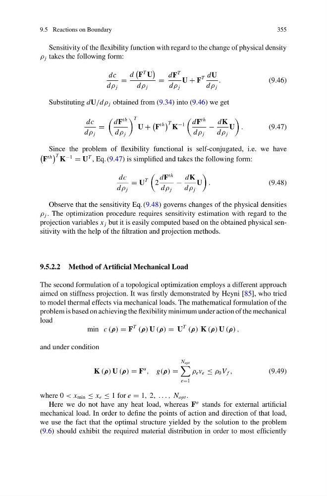
Sensitivity of the flexibility function with regard to the change of physical density
ρ j takes the following form:
dc
dρ j
=
d
F
T U
dρ j
=
dF
T
dρ j
U + F
T dU
dρ j
.
(9.46)
Substituting dU/dρ j obtained from (9.34) into (9.46) we get
dc
dρ j
=
dF
th
dρ j
T
U +
F
th
T K
−1
dF
th
dρ j
−
dK
dρ j
U
.
(9.47)
Since the problem of flexibility functional is self-conjugated, i.e. we have
F
th
T K
−1
= U
T , Eq. (9.47) is simplified and takes the following form:
dc
dρ j
= U
T
2
dF
th
dρ j
−
dK
dρ j
U
.
(9.48)
Observe that the sensitivity Eq. (9.48) governs changes of the physical densities
ρ j . The optimization procedure requires sensitivity estimation with regard to the
projection variables x j but it is easily computed based on the obtained physical sensitivity with the help of the filtration and projection methods.
9.5.2.2 Method of Artificial Mechanical Load
The second formulation of a topological optimization employs a different approach
aimed on stiffness projection. It was firstly demonstrated by Heyni [85], who tried
to model thermal effects via mechanical loads. The mathematical formulation of the
problem is based on achieving the flexibility minimum under action of the mechanical
load
min c (ρ) = F
T
(ρ) U (ρ) = U
T
(ρ) K (ρ) U (ρ) ,
and under condition
K (ρ) U (ρ) = F
a
, g(ρ) =
N opt
e=1
ρ e v e ≤ ρ 0 V f ,
(9.49)
where 0 < x min ≤ x e ≤ 1 for e = 1, 2, . . . , N opt .
Here we do not have any heat load, whereas F
a stands for external artificial
mechanical load. In order to define the points of action and direction of that load,
we use the fact that the optimal structure yielded by the solution to the problem
(9.6) should exhibit the required material distribution in order to most efficiently
355
Sensitivity of the flexibility function with regard to the change of physical density
ρ j takes the following form:
dc
dρ j
=
d
F
T U
dρ j
=
dF
T
dρ j
U + F
T dU
dρ j
.
(9.46)
Substituting dU/dρ j obtained from (9.34) into (9.46) we get
dc
dρ j
=
dF
th
dρ j
T
U +
F
th
T K
−1
dF
th
dρ j
−
dK
dρ j
U
.
(9.47)
Since the problem of flexibility functional is self-conjugated, i.e. we have
F
th
T K
−1
= U
T , Eq. (9.47) is simplified and takes the following form:
dc
dρ j
= U
T
2
dF
th
dρ j
−
dK
dρ j
U
.
(9.48)
Observe that the sensitivity Eq. (9.48) governs changes of the physical densities
ρ j . The optimization procedure requires sensitivity estimation with regard to the
projection variables x j but it is easily computed based on the obtained physical sensitivity with the help of the filtration and projection methods.
9.5.2.2 Method of Artificial Mechanical Load
The second formulation of a topological optimization employs a different approach
aimed on stiffness projection. It was firstly demonstrated by Heyni [85], who tried
to model thermal effects via mechanical loads. The mathematical formulation of the
problem is based on achieving the flexibility minimum under action of the mechanical
load
min c (ρ) = F
T
(ρ) U (ρ) = U
T
(ρ) K (ρ) U (ρ) ,
and under condition
K (ρ) U (ρ) = F
a
, g(ρ) =
N opt
e=1
ρ e v e ≤ ρ 0 V f ,
(9.49)
where 0 < x min ≤ x e ≤ 1 for e = 1, 2, . . . , N opt .
Here we do not have any heat load, whereas F
a stands for external artificial
mechanical load. In order to define the points of action and direction of that load,
we use the fact that the optimal structure yielded by the solution to the problem
(9.6) should exhibit the required material distribution in order to most efficiently