

278
7 Mathematical Models of Functionally Graded Beams in Temperature Field
β =
12G 3 t 3 (1 − ϑ)
Eγ 2
.
(7.162)
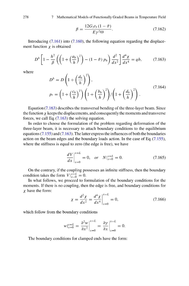
Introducing (7.161) into (7.160), the following equation regarding the displacement function χ is obtained
D
h
1 −
h
2
β
1 +
a h
h
2
− (1 − ϑ) p h
d
2
dx 2
d
4
χ
dx 4 = qb,
(7.163)
where
D
h
= D
1 +
d h
h
2
,
ph =
1 +
c h
h
2
1 +
b h
h
2
/
1 +
d h
h
2
.
(7.164)
Equation (7.163) describes the transversal bending of the three-layer beam. Since
the function χ keeps the displacements, and consequently the moments and transverse
forces, we call Eq. (7.163) the solving equation.
In order to choose the formulation of the problem regarding deformation of the
three-layer beam, it is necessary to attach boundary conditions to the equilibrium
equations (7.155) and (7.163). The latter express the influences of both the boundaries
action on the beam edges and the boundary loads action. In the case of Eq. (7.155),
where the stiffness is equal to zero (the edge is free), we have
dV
dx
x=L
x=0
= 0, or N |
x=L
x=0 = 0.
(7.165)
On the contrary, if the coupling possesses an infinite stiffness, then the boundary
condition takes the form V |
x=L
x=0 = 0.
In what follows, we proceed to formulation of the boundary conditions for the
moments. If there is no coupling, then the edge is free, and boundary conditions for
χ have the form:
χ =
d
2
χ
dx 2 =
d
4
χ
dx 4
x=L
x=0
= 0,
(7.166)
which follow from the boundary conditions
w|
x=L
x=0 =
∂
2 w
∂ x 2
x=L
x=0
=
∂γ
∂ x
x=L
x=0
= 0.
The boundary conditions for clamped ends have the form:
7 Mathematical Models of Functionally Graded Beams in Temperature Field
β =
12G 3 t 3 (1 − ϑ)
Eγ 2
.
(7.162)
Introducing (7.161) into (7.160), the following equation regarding the displacement function χ is obtained
D
h
1 −
h
2
β
1 +
a h
h
2
− (1 − ϑ) p h
d
2
dx 2
d
4
χ
dx 4 = qb,
(7.163)
where
D
h
= D
1 +
d h
h
2
,
ph =
1 +
c h
h
2
1 +
b h
h
2
/
1 +
d h
h
2
.
(7.164)
Equation (7.163) describes the transversal bending of the three-layer beam. Since
the function χ keeps the displacements, and consequently the moments and transverse
forces, we call Eq. (7.163) the solving equation.
In order to choose the formulation of the problem regarding deformation of the
three-layer beam, it is necessary to attach boundary conditions to the equilibrium
equations (7.155) and (7.163). The latter express the influences of both the boundaries
action on the beam edges and the boundary loads action. In the case of Eq. (7.155),
where the stiffness is equal to zero (the edge is free), we have
dV
dx
x=L
x=0
= 0, or N |
x=L
x=0 = 0.
(7.165)
On the contrary, if the coupling possesses an infinite stiffness, then the boundary
condition takes the form V |
x=L
x=0 = 0.
In what follows, we proceed to formulation of the boundary conditions for the
moments. If there is no coupling, then the edge is free, and boundary conditions for
χ have the form:
χ =
d
2
χ
dx 2 =
d
4
χ
dx 4
x=L
x=0
= 0,
(7.166)
which follow from the boundary conditions
w|
x=L
x=0 =
∂
2 w
∂ x 2
x=L
x=0
=
∂γ
∂ x
x=L
x=0
= 0.
The boundary conditions for clamped ends have the form: