

276
7 Mathematical Models of Functionally Graded Beams in Temperature Field
N p = b
c+h 1
−c−h 2
σ p dz, Q p = b
c+h 1
−c−h 2
τ p dz, M p = b
c+h 1
−c−h 2
zσ p dz −
1
2
hc 13 N p ,
(7.151)
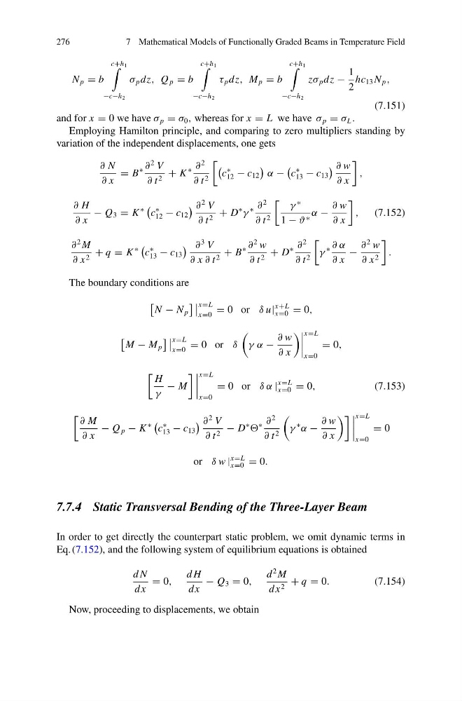
and for x = 0 we have σ p = σ 0 , whereas for x = L we have σ p = σ L .
Employing Hamilton principle, and comparing to zero multipliers standing by
variation of the independent displacements, one gets
∂ N
∂ x
= B
∗ ∂
2 V
∂ t 2 + K
∗ ∂
2
∂ t 2
c
∗
12 − c 12
α −
c
∗
13 − c 13
∂ w
∂ x
,
∂ H
∂ x
− Q 3 = K
∗
c
∗
12 − c 12
∂
2 V
∂ t 2 + D
∗
γ
∗ ∂
2
∂ t 2
γ
∗
1 − ϑ ∗ α −
∂ w
∂ x
, (7.152)
∂
2 M
∂ x 2 + q = K
∗
c
∗
13 − c 13
∂
3 V
∂ x ∂ t 2 + B
∗ ∂
2 w
∂ t 2 + D
∗ ∂
2
∂ t 2
γ
∗ ∂ α
∂ x
−
∂
2 w
∂ x 2
.
The boundary conditions are
N − N p
x=L
x=0
= 0 or δ u|
x+L
x=0 = 0,
M − M p
x=L
x=0
= 0 or δ
γ α −
∂ w
∂ x
x=L
x=0
= 0,
H
γ
− M
x=L
x=0
= 0 or δ α |
x=L
x=0 = 0,
(7.153)
∂ M
∂ x
− Q p − K
∗
c
∗
13 − c 13
∂
2 V
∂ t 2 − D
∗
∗ ∂
2
∂ t 2
γ
∗
α −
∂ w
∂ x
x=L
x=0
= 0
or δ w |
x=L
x=0 = 0.
7.7.4 Static Transversal Bending of the Three-Layer Beam
In order to get directly the counterpart static problem, we omit dynamic terms in
Eq. (7.152), and the following system of equilibrium equations is obtained
d N
dx
= 0,
d H
dx
− Q 3 = 0,
d
2 M
dx 2 + q = 0.
(7.154)
Now, proceeding to displacements, we obtain
7 Mathematical Models of Functionally Graded Beams in Temperature Field
N p = b
c+h 1
−c−h 2
σ p dz, Q p = b
c+h 1
−c−h 2
τ p dz, M p = b
c+h 1
−c−h 2
zσ p dz −
1
2
hc 13 N p ,
(7.151)
and for x = 0 we have σ p = σ 0 , whereas for x = L we have σ p = σ L .
Employing Hamilton principle, and comparing to zero multipliers standing by
variation of the independent displacements, one gets
∂ N
∂ x
= B
∗ ∂
2 V
∂ t 2 + K
∗ ∂
2
∂ t 2
c
∗
12 − c 12
α −
c
∗
13 − c 13
∂ w
∂ x
,
∂ H
∂ x
− Q 3 = K
∗
c
∗
12 − c 12
∂
2 V
∂ t 2 + D
∗
γ
∗ ∂
2
∂ t 2
γ
∗
1 − ϑ ∗ α −
∂ w
∂ x
, (7.152)
∂
2 M
∂ x 2 + q = K
∗
c
∗
13 − c 13
∂
3 V
∂ x ∂ t 2 + B
∗ ∂
2 w
∂ t 2 + D
∗ ∂
2
∂ t 2
γ
∗ ∂ α
∂ x
−
∂
2 w
∂ x 2
.
The boundary conditions are
N − N p
x=L
x=0
= 0 or δ u|
x+L
x=0 = 0,
M − M p
x=L
x=0
= 0 or δ
γ α −
∂ w
∂ x
x=L
x=0
= 0,
H
γ
− M
x=L
x=0
= 0 or δ α |
x=L
x=0 = 0,
(7.153)
∂ M
∂ x
− Q p − K
∗
c
∗
13 − c 13
∂
2 V
∂ t 2 − D
∗
∗ ∂
2
∂ t 2
γ
∗
α −
∂ w
∂ x
x=L
x=0
= 0
or δ w |
x=L
x=0 = 0.
7.7.4 Static Transversal Bending of the Three-Layer Beam
In order to get directly the counterpart static problem, we omit dynamic terms in
Eq. (7.152), and the following system of equilibrium equations is obtained
d N
dx
= 0,
d H
dx
− Q 3 = 0,
d
2 M
dx 2 + q = 0.
(7.154)
Now, proceeding to displacements, we obtain