

7.6 Stability of Curvilinear Euler-Bernoulli Beams in Temperature Fields
251
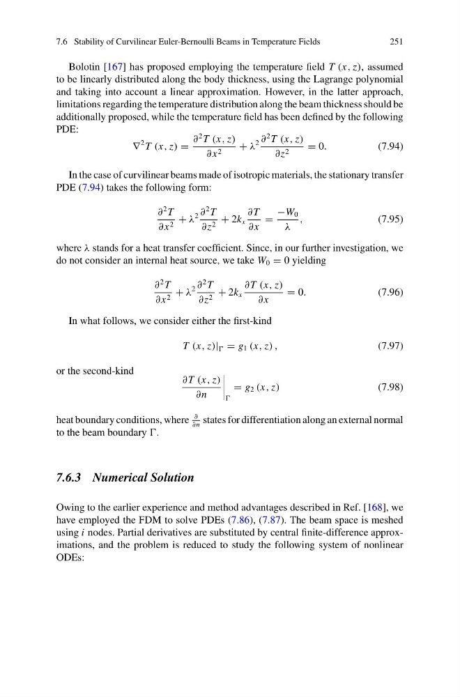
Bolotin [167] has proposed employing the temperature field T (x, z), assumed
to be linearly distributed along the body thickness, using the Lagrange polynomial
and taking into account a linear approximation. However, in the latter approach,
limitations regarding the temperature distribution along the beam thickness should be
additionally proposed, while the temperature field has been defined by the following
PDE:
∇
2 T (x, z) =
∂
2 T (x, z)
∂ x 2
+ λ
2 ∂
2 T (x, z)
∂z 2
= 0.
(7.94)
In the case of curvilinear beams made of isotropic materials, the stationary transfer
PDE (7.94) takes the following form:
∂
2 T
∂ x 2 + λ
2 ∂
2 T
∂z 2 + 2k x
∂ T
∂ x
=
−W 0
λ
,
(7.95)
where λ stands for a heat transfer coefficient. Since, in our further investigation, we
do not consider an internal heat source, we take W 0 = 0 yielding
∂
2 T
∂ x 2 + λ
2 ∂
2 T
∂z 2 + 2k x
∂ T (x, z)
∂ x
= 0.
(7.96)
In what follows, we consider either the first-kind
T (x, z)| = g 1 (x, z) ,
(7.97)
or the second-kind
∂ T (x, z)
∂n
= g 2 (x, z)
(7.98)
heat boundary conditions, where
∂
∂n
states for differentiation along an external normal
to the beam boundary .
7.6.3 Numerical Solution
Owing to the earlier experience and method advantages described in Ref. [168], we
have employed the FDM to solve PDEs (7.86), (7.87). The beam space is meshed
using i nodes. Partial derivatives are substituted by central finite-difference approximations, and the problem is reduced to study the following system of nonlinear
ODEs:
251
Bolotin [167] has proposed employing the temperature field T (x, z), assumed
to be linearly distributed along the body thickness, using the Lagrange polynomial
and taking into account a linear approximation. However, in the latter approach,
limitations regarding the temperature distribution along the beam thickness should be
additionally proposed, while the temperature field has been defined by the following
PDE:
∇
2 T (x, z) =
∂
2 T (x, z)
∂ x 2
+ λ
2 ∂
2 T (x, z)
∂z 2
= 0.
(7.94)
In the case of curvilinear beams made of isotropic materials, the stationary transfer
PDE (7.94) takes the following form:
∂
2 T
∂ x 2 + λ
2 ∂
2 T
∂z 2 + 2k x
∂ T
∂ x
=
−W 0
λ
,
(7.95)
where λ stands for a heat transfer coefficient. Since, in our further investigation, we
do not consider an internal heat source, we take W 0 = 0 yielding
∂
2 T
∂ x 2 + λ
2 ∂
2 T
∂z 2 + 2k x
∂ T (x, z)
∂ x
= 0.
(7.96)
In what follows, we consider either the first-kind
T (x, z)| = g 1 (x, z) ,
(7.97)
or the second-kind
∂ T (x, z)
∂n
= g 2 (x, z)
(7.98)
heat boundary conditions, where
∂
∂n
states for differentiation along an external normal
to the beam boundary .
7.6.3 Numerical Solution
Owing to the earlier experience and method advantages described in Ref. [168], we
have employed the FDM to solve PDEs (7.86), (7.87). The beam space is meshed
using i nodes. Partial derivatives are substituted by central finite-difference approximations, and the problem is reduced to study the following system of nonlinear
ODEs: