

236
7 Mathematical Models of Functionally Graded Beams in Temperature Field
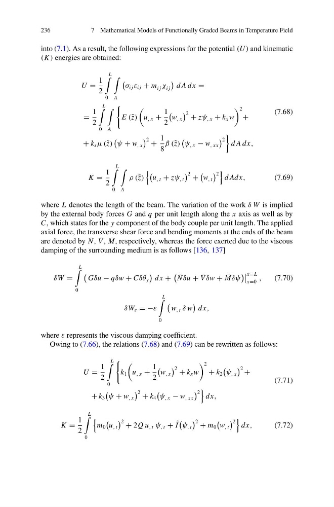
into (7.1). As a result, the following expressions for the potential (U ) and kinematic
(K ) energies are obtained:
U =
1
2
L
0
A
σ i j ε i j + m i j χ i j
d A dx =
=
1
2
L
0
A
E (˜ z)
u , x +
1
2
w , x
2 + zψ , x + k x w
2
+
+ k s μ (˜ z)
ψ + w , x
2 +
1
8
β (˜ z)
ψ , x − w , xx
2
d A dx,
(7.68)
K =
1
2
L
0
A
ρ (˜ z)
u , t + zψ , t
2 +
w , t
2
d Adx,
(7.69)
where L denotes the length of the beam. The variation of the work δ W is implied
by the external body forces G and q per unit length along the x axis as well as by
C, which states for the y component of the body couple per unit length. The applied
axial force, the transverse shear force and bending moments at the ends of the beam
are denoted by ¯
N , ¯
V , ¯
M, respectively, whereas the force exerted due to the viscous
damping of the surrounding medium is as follows [136, 137]
δW =
L
0
Gδu − qδw + Cδθ y
dx +
¯
N δu + ¯
V δw + ¯
Mδψ
x=L
x=0
,
(7.70)
δW ε = −ε
L
0
w , t δ w
dx,
where ε represents the viscous damping coefficient.
Owing to (7.66), the relations (7.68) and (7.69) can be rewritten as follows:
U =
1
2
L
0
k 1
u , x +
1
2
w , x
2 + k x w
2
+ k 2
ψ , x
2 +
+ k 3
ψ + w , x
2 + k 4
ψ , x − w , xx
2
dx,
(7.71)
K =
1
2
L
0
m 0
u , t
2 + 2Q u , t ψ , t + ˜
I
ψ , t
2 + m 0
w , t
2
dx,
(7.72)
7 Mathematical Models of Functionally Graded Beams in Temperature Field
into (7.1). As a result, the following expressions for the potential (U ) and kinematic
(K ) energies are obtained:
U =
1
2
L
0
A
σ i j ε i j + m i j χ i j
d A dx =
=
1
2
L
0
A
E (˜ z)
u , x +
1
2
w , x
2 + zψ , x + k x w
2
+
+ k s μ (˜ z)
ψ + w , x
2 +
1
8
β (˜ z)
ψ , x − w , xx
2
d A dx,
(7.68)
K =
1
2
L
0
A
ρ (˜ z)
u , t + zψ , t
2 +
w , t
2
d Adx,
(7.69)
where L denotes the length of the beam. The variation of the work δ W is implied
by the external body forces G and q per unit length along the x axis as well as by
C, which states for the y component of the body couple per unit length. The applied
axial force, the transverse shear force and bending moments at the ends of the beam
are denoted by ¯
N , ¯
V , ¯
M, respectively, whereas the force exerted due to the viscous
damping of the surrounding medium is as follows [136, 137]
δW =
L
0
Gδu − qδw + Cδθ y
dx +
¯
N δu + ¯
V δw + ¯
Mδψ
x=L
x=0
,
(7.70)
δW ε = −ε
L
0
w , t δ w
dx,
where ε represents the viscous damping coefficient.
Owing to (7.66), the relations (7.68) and (7.69) can be rewritten as follows:
U =
1
2
L
0
k 1
u , x +
1
2
w , x
2 + k x w
2
+ k 2
ψ , x
2 +
+ k 3
ψ + w , x
2 + k 4
ψ , x − w , xx
2
dx,
(7.71)
K =
1
2
L
0
m 0
u , t
2 + 2Q u , t ψ , t + ˜
I
ψ , t
2 + m 0
w , t
2
dx,
(7.72)