

6.6 Chaotic Dynamics of the Size-Dependent Flexible Beams
179
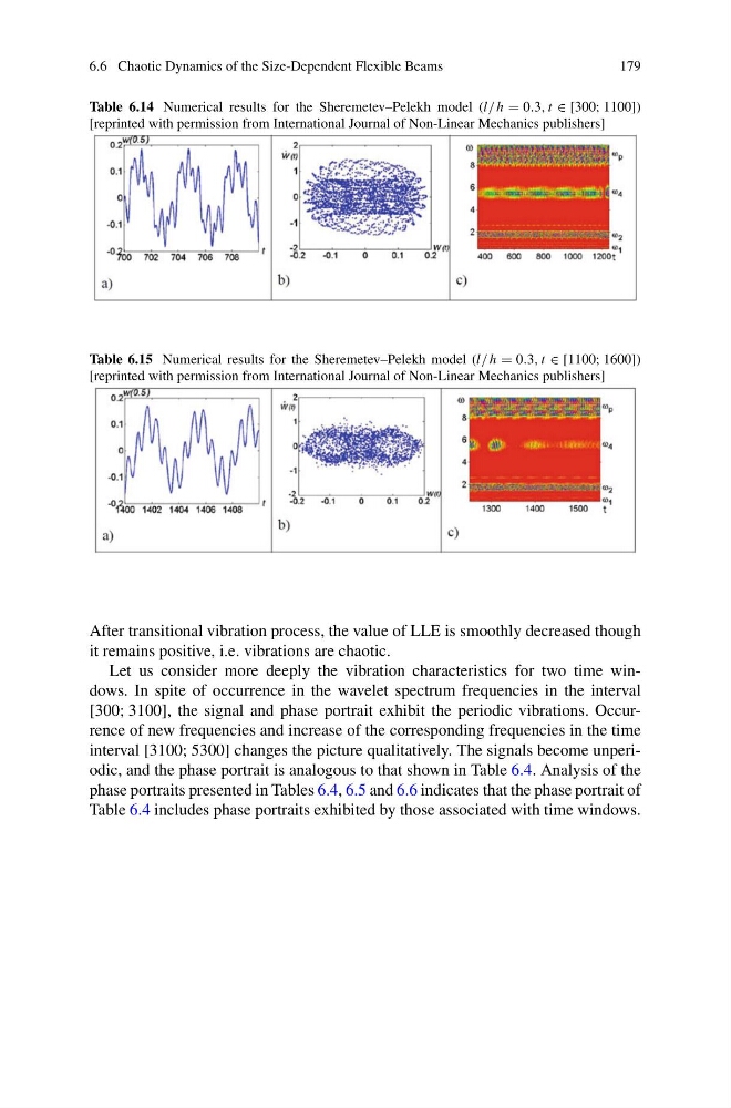
Table 6.14 Numerical results for the Sheremetev–Pelekh model (l/ h = 0.3, t ∈ [300; 1100])
[reprinted with permission from International Journal of Non-Linear Mechanics publishers]
Table 6.15 Numerical results for the Sheremetev–Pelekh model (l/ h = 0.3, t ∈ [1100; 1600])
[reprinted with permission from International Journal of Non-Linear Mechanics publishers]
After transitional vibration process, the value of LLE is smoothly decreased though
it remains positive, i.e. vibrations are chaotic.
Let us consider more deeply the vibration characteristics for two time windows. In spite of occurrence in the wavelet spectrum frequencies in the interval
[300; 3100], the signal and phase portrait exhibit the periodic vibrations. Occurrence of new frequencies and increase of the corresponding frequencies in the time
interval [3100; 5300] changes the picture qualitatively. The signals become unperiodic, and the phase portrait is analogous to that shown in Table 6.4. Analysis of the
phase portraits presented in Tables 6.4, 6.5 and 6.6 indicates that the phase portrait of
Table 6.4 includes phase portraits exhibited by those associated with time windows.
179
Table 6.14 Numerical results for the Sheremetev–Pelekh model (l/ h = 0.3, t ∈ [300; 1100])
[reprinted with permission from International Journal of Non-Linear Mechanics publishers]
Table 6.15 Numerical results for the Sheremetev–Pelekh model (l/ h = 0.3, t ∈ [1100; 1600])
[reprinted with permission from International Journal of Non-Linear Mechanics publishers]
After transitional vibration process, the value of LLE is smoothly decreased though
it remains positive, i.e. vibrations are chaotic.
Let us consider more deeply the vibration characteristics for two time windows. In spite of occurrence in the wavelet spectrum frequencies in the interval
[300; 3100], the signal and phase portrait exhibit the periodic vibrations. Occurrence of new frequencies and increase of the corresponding frequencies in the time
interval [3100; 5300] changes the picture qualitatively. The signals become unperiodic, and the phase portrait is analogous to that shown in Table 6.4. Analysis of the
phase portraits presented in Tables 6.4, 6.5 and 6.6 indicates that the phase portrait of
Table 6.4 includes phase portraits exhibited by those associated with time windows.