

6.4 Technical Theory for the Different Models
155
panel then B i = 0 (i = 1, . . . , 4), J 1 = J 3 = J 5 = 0, I 1 = I 3 = I 5 = 0. In this case
the resolving Eqs. (6.68)–(6.70) and the corresponding boundary conditions (6.71)–
(6.74) coincide with the classical Sheremetev–Pelekh equations [53]. The obtained
equations of motion are general, i.e. they imply the Timoshenko and Bernoulli–Euler
equations with/without the size-dependent behaviour.
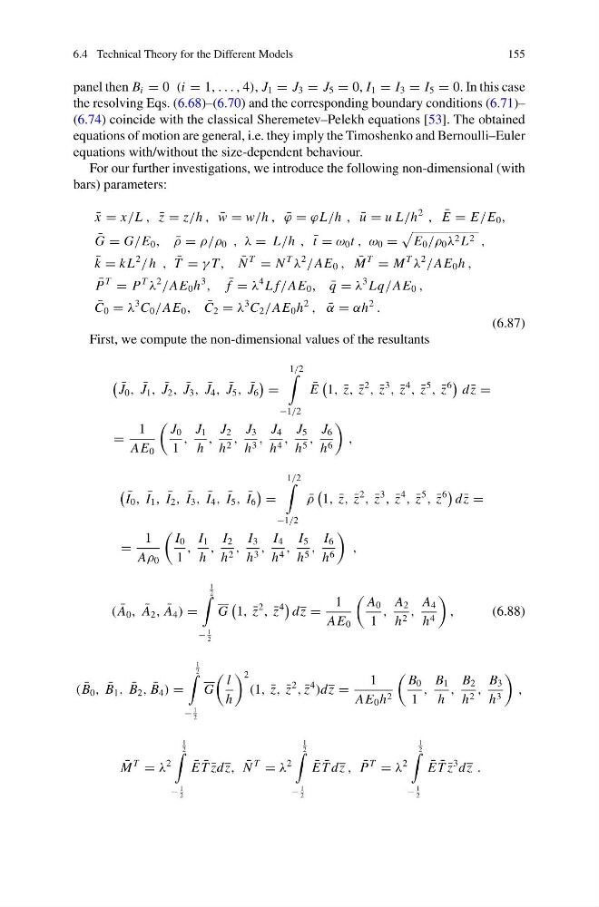
For our further investigations, we introduce the following non-dimensional (with
bars) parameters:
¯
x = x/L , ¯
z = z/h , ¯
w = w/h , ¯
ϕ = ϕ L/h , ¯
u = u L/h
2
, ¯
E = E/E 0 ,
¯
G = G/E 0 , ¯
ρ = ρ/ρ 0 , λ = L/h , ¯
t = ω 0 t , ω 0 =
E 0 /ρ 0 λ 2 L 2 ,
¯
k = k L
2
/ h , ¯
T = γ T, ¯
N
T
= N
T
λ
2
/AE 0 , ¯
M
T
= M
T
λ
2
/AE 0 h ,
¯
P
T
= P
T
λ
2
/AE 0 h
3
, ¯
f = λ
4 L f/AE 0 , ¯
q = λ
3 Lq/AE 0 ,
¯
C 0 = λ
3 C 0 /AE 0 , ¯
C 2 = λ
3 C 2 /AE 0 h
2
, ¯
α = αh
2
.
(6.87)
First, we compute the non-dimensional values of the resultants
¯
J 0 , ¯
J 1 , ¯
J 2 , ¯
J 3 , ¯
J 4 , ¯
J 5 , ¯
J 6
=
1/2
−1/2
¯
E
1, ¯
z, ¯
z
2
, ¯
z
3
, ¯
z
4
, ¯
z
5
, ¯
z
6
d ¯
z =
=
1
AE 0
J 0
1
,
J 1
h
,
J 2
h 2 ,
J 3
h 3 ,
J 4
h 4 ,
J 5
h 5 ,
J 6
h 6
,
¯
I 0 , ¯
I 1 , ¯
I 2 , ¯
I 3 , ¯
I 4 , ¯
I 5 , ¯
I 6
=
1/2
−1/2
¯
ρ
1, ¯
z, ¯
z
2
, ¯
z
3
, ¯
z
4
, ¯
z
5
, ¯
z
6
d ¯
z =
=
1
Aρ 0
I 0
1
,
I 1
h
,
I 2
h 2 ,
I 3
h 3 ,
I 4
h 4 ,
I 5
h 5 ,
I 6
h 6
,
( ¯
A 0 , ¯
A 2 , ¯
A 4 ) =
1
2
−
1
2
G
1, ¯
z
2
, ¯
z
4
dz =
1
AE 0
A 0
1
,
A 2
h 2 ,
A 4
h 4
,
(6.88)
( ¯
B 0 , ¯
B 1 , ¯
B 2 , ¯
B 4 ) =
1
2
−
1
2
G
l
h
2
(1, ¯
z, ¯
z
2
, ¯
z
4
)dz =
1
AE 0 h 2
B 0
1
,
B 1
h
,
B 2
h 2 ,
B 3
h 3
,
¯
M
T
= λ
2
1
2
−
1
2
¯
E ¯
T ¯
zdz, ¯
N
T
= λ
2
1
2
−
1
2
¯
E ¯
T dz , ¯
P
T
= λ
2
1
2
−
1
2
¯
E ¯
T ¯
z
3 dz .
155
panel then B i = 0 (i = 1, . . . , 4), J 1 = J 3 = J 5 = 0, I 1 = I 3 = I 5 = 0. In this case
the resolving Eqs. (6.68)–(6.70) and the corresponding boundary conditions (6.71)–
(6.74) coincide with the classical Sheremetev–Pelekh equations [53]. The obtained
equations of motion are general, i.e. they imply the Timoshenko and Bernoulli–Euler
equations with/without the size-dependent behaviour.
For our further investigations, we introduce the following non-dimensional (with
bars) parameters:
¯
x = x/L , ¯
z = z/h , ¯
w = w/h , ¯
ϕ = ϕ L/h , ¯
u = u L/h
2
, ¯
E = E/E 0 ,
¯
G = G/E 0 , ¯
ρ = ρ/ρ 0 , λ = L/h , ¯
t = ω 0 t , ω 0 =
E 0 /ρ 0 λ 2 L 2 ,
¯
k = k L
2
/ h , ¯
T = γ T, ¯
N
T
= N
T
λ
2
/AE 0 , ¯
M
T
= M
T
λ
2
/AE 0 h ,
¯
P
T
= P
T
λ
2
/AE 0 h
3
, ¯
f = λ
4 L f/AE 0 , ¯
q = λ
3 Lq/AE 0 ,
¯
C 0 = λ
3 C 0 /AE 0 , ¯
C 2 = λ
3 C 2 /AE 0 h
2
, ¯
α = αh
2
.
(6.87)
First, we compute the non-dimensional values of the resultants
¯
J 0 , ¯
J 1 , ¯
J 2 , ¯
J 3 , ¯
J 4 , ¯
J 5 , ¯
J 6
=
1/2
−1/2
¯
E
1, ¯
z, ¯
z
2
, ¯
z
3
, ¯
z
4
, ¯
z
5
, ¯
z
6
d ¯
z =
=
1
AE 0
J 0
1
,
J 1
h
,
J 2
h 2 ,
J 3
h 3 ,
J 4
h 4 ,
J 5
h 5 ,
J 6
h 6
,
¯
I 0 , ¯
I 1 , ¯
I 2 , ¯
I 3 , ¯
I 4 , ¯
I 5 , ¯
I 6
=
1/2
−1/2
¯
ρ
1, ¯
z, ¯
z
2
, ¯
z
3
, ¯
z
4
, ¯
z
5
, ¯
z
6
d ¯
z =
=
1
Aρ 0
I 0
1
,
I 1
h
,
I 2
h 2 ,
I 3
h 3 ,
I 4
h 4 ,
I 5
h 5 ,
I 6
h 6
,
( ¯
A 0 , ¯
A 2 , ¯
A 4 ) =
1
2
−
1
2
G
1, ¯
z
2
, ¯
z
4
dz =
1
AE 0
A 0
1
,
A 2
h 2 ,
A 4
h 4
,
(6.88)
( ¯
B 0 , ¯
B 1 , ¯
B 2 , ¯
B 4 ) =
1
2
−
1
2
G
l
h
2
(1, ¯
z, ¯
z
2
, ¯
z
4
)dz =
1
AE 0 h 2
B 0
1
,
B 1
h
,
B 2
h 2 ,
B 3
h 3
,
¯
M
T
= λ
2
1
2
−
1
2
¯
E ¯
T ¯
zdz, ¯
N
T
= λ
2
1
2
−
1
2
¯
E ¯
T dz , ¯
P
T
= λ
2
1
2
−
1
2
¯
E ¯
T ¯
z
3 dz .