

318
M. Parikh et al.
RMS =
[h a (t) − h e (t)]
2
n
(6)
where h a (t) is actual contact conductance and h e (t) is the estimated value of contact
conductance. Figure 4a shows a sample of comparison for the estimation of step
contact conductance h(t) profile with different population cases. It is found that
RMS error for 30 and 50 populations is nearly similar, but the computational time
has a large variation which make 30 populations size good for estimation. Figure 4b
shows a sample of comparison for the estimation of step contact conductance h(t)
profile with different measurement errors. It is observed that the measurement error
is directly proportional to RMS error. Figure 5a, b show the results for the estimation
of double triangular profile and linear profile of heat flux, respectively. Satisfactory
results were obtained for these profiles also which suggest that the Jaya algorithm
can estimate any heat flux profile very accurately.
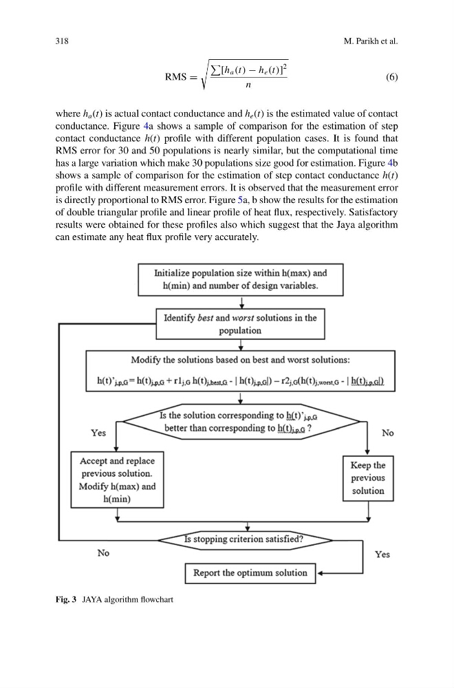
Fig. 3 JAYA algorithm flowchart
M. Parikh et al.
RMS =
[h a (t) − h e (t)]
2
n
(6)
where h a (t) is actual contact conductance and h e (t) is the estimated value of contact
conductance. Figure 4a shows a sample of comparison for the estimation of step
contact conductance h(t) profile with different population cases. It is found that
RMS error for 30 and 50 populations is nearly similar, but the computational time
has a large variation which make 30 populations size good for estimation. Figure 4b
shows a sample of comparison for the estimation of step contact conductance h(t)
profile with different measurement errors. It is observed that the measurement error
is directly proportional to RMS error. Figure 5a, b show the results for the estimation
of double triangular profile and linear profile of heat flux, respectively. Satisfactory
results were obtained for these profiles also which suggest that the Jaya algorithm
can estimate any heat flux profile very accurately.
Fig. 3 JAYA algorithm flowchart