

x 1
ffiffiffiffiffi ffi
K 1
p % 1:57080 c; x 2
ffiffiffiffiffi ffi
K 2
p % 5:05297 c:
ð2:89Þ
Comparing to the exact values x 1 = pc/2 % 1.57079c and x 2 = 3pc/2 %
4.71238c, the first estimate is very close to the true first eigenvalue x 1 , whereas the
second is 7% in error. Using more test functions improves the quality of all
eigenvalue estimates. Thus if only v 1 is employed, the estimate of x 1 changes to
x 1
√(5/2)c % 1.581, clearly less accurate than the estimate obtained using both
v 1 and v 2 .
2.8.4 The Finite Difference Method
Finite difference methods rely on approximating infinitely small differentials by
finite-magnitude differences. Differential equations will then transform into difference equations. Finite difference methods are applicable to any type of boundary
value and/or initial value problem, including those associated with partial and/or
nonlinear differential equations. The methods are easily automated, and thus
especially well suited to computer applications.
Here we illustrate a simple central-difference scheme for solving differential
EVPs; Extensions and variants of the method are described in, e.g. Collatz (1963),
Flügge (1962), and Press et al. (2002).
For an EVP with a given ordinary differential equation, one divides the x-interval
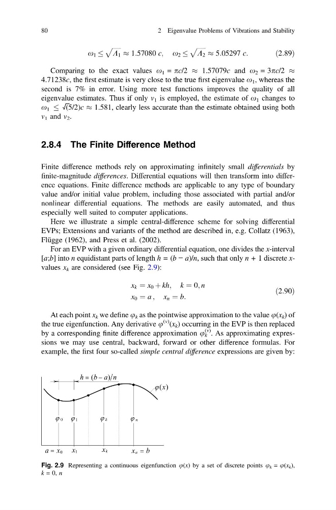
[a;b] into n equidistant parts of length h = (b − a)/n, such that only n + 1 discrete xvalues x k are considered (see Fig. 2.9):
x k ¼ x 0 þ kh; k ¼ 0; n
x 0 ¼ a ; x n ¼ b:
ð2:90Þ
At each point x k we define u k as the pointwise approximation to the value u(x k ) of
the true eigenfunction. Any derivative u
(m) (x k ) occurring in the EVP is then replaced
by a corresponding finite difference approximation u k
(m) . As approximating expressions we may use central, backward, forward or other difference formulas. For
example, the first four so-called simple central difference expressions are given by:
Fig. 2.9 Representing a continuous eigenfunction u(x) by a set of discrete points u k = u(x k ),
k = 0, n
80
2 Eigenvalue Problems of Vibrations and Stability
ffiffiffiffiffi ffi
K 1
p % 1:57080 c; x 2
ffiffiffiffiffi ffi
K 2
p % 5:05297 c:
ð2:89Þ
Comparing to the exact values x 1 = pc/2 % 1.57079c and x 2 = 3pc/2 %
4.71238c, the first estimate is very close to the true first eigenvalue x 1 , whereas the
second is 7% in error. Using more test functions improves the quality of all
eigenvalue estimates. Thus if only v 1 is employed, the estimate of x 1 changes to
x 1
√(5/2)c % 1.581, clearly less accurate than the estimate obtained using both
v 1 and v 2 .
2.8.4 The Finite Difference Method
Finite difference methods rely on approximating infinitely small differentials by
finite-magnitude differences. Differential equations will then transform into difference equations. Finite difference methods are applicable to any type of boundary
value and/or initial value problem, including those associated with partial and/or
nonlinear differential equations. The methods are easily automated, and thus
especially well suited to computer applications.
Here we illustrate a simple central-difference scheme for solving differential
EVPs; Extensions and variants of the method are described in, e.g. Collatz (1963),
Flügge (1962), and Press et al. (2002).
For an EVP with a given ordinary differential equation, one divides the x-interval
[a;b] into n equidistant parts of length h = (b − a)/n, such that only n + 1 discrete xvalues x k are considered (see Fig. 2.9):
x k ¼ x 0 þ kh; k ¼ 0; n
x 0 ¼ a ; x n ¼ b:
ð2:90Þ
At each point x k we define u k as the pointwise approximation to the value u(x k ) of
the true eigenfunction. Any derivative u
(m) (x k ) occurring in the EVP is then replaced
by a corresponding finite difference approximation u k
(m) . As approximating expressions we may use central, backward, forward or other difference formulas. For
example, the first four so-called simple central difference expressions are given by:
Fig. 2.9 Representing a continuous eigenfunction u(x) by a set of discrete points u k = u(x k ),
k = 0, n
80
2 Eigenvalue Problems of Vibrations and Stability