

Summarizing we have:
Rayleigh–Ritz Method. For a differential EVP Ku = kLu:
1. Choose a set of test functions v j (x)2u TF , j = 1, q
2. Compute matrices K and L, with components k ij and l ij as given by (2.81)
3. Solve the algebraic EVP Ka = KLa for the eigenvalues K j , j = 1, q
If Ku = kLu is self-adjoint and completely definite, then k j
K j for
j = 1, q.
The quality of eigenvalue estimates – in particular the higher ones – strongly
depends on the number and quality of selected test functions. Most test functions
will yield a fair approximation to at least the lowest eigenvalue. However, it is
generally recommended to select test functions that qualitatively resemble the
assumed true eigenfunctions. If this is impossible, one should choose q ) n, where
n is the number of eigenvalues to be estimated.
The Rayleigh–Ritz method is incapable of providing lower-bound estimates;
Temple quotients may be useful for this purpose (Collatz 1963).
Example 2.19. The EVP associated with vibrations of an elastic rod of length
l = 1 is −c
2 u′′ = x
2 u with u(0) = u′(1) = 0. The EVP is self-adjoint and completely definite (cf. Examples 2.8 and 2.10). We here employ Rayleigh–Ritz’s
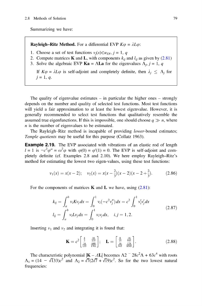
method for estimating the lowest two eigen-values, using these test functions:
v 1 ðxÞ ¼ xðx À 2Þ; v 2 ðxÞ ¼ xðx À
2
3
Þðx À 2Þðx À 2 þ
2
3
Þ:
ð2:86Þ
For the components of matrices K and L we have, using (2.81):
k ij ¼
Z b
a
v i Kv j dx ¼
Z 1
0
v i ðÀc
2 v
00
j Þdx ¼ c
2
Z 1
0
v
0
i v
0
j dx
l ij ¼
Z b
a
v i Lv j dx ¼
Z 1
0
v i v j dx; i; j ¼ 1; 2:
ð2:87Þ
Inserting v 1 and v 2 and integrating it is found that:
K ¼ c
2
4
3
16
135
16
135
640
1701
!
; L ¼
8
15
16
945
16
945
128
8505
!
:
ð2:88Þ
The characteristic polynomial |K – KL| becomes K2
− 28c
2
K + 63c
4 with roots
K 1 = (14 − √133)c
2 and K 2 = √7(2√7 + √19)c
2 . So for the two lowest natural
frequencies:
2.8 Methods of Solution
79
Rayleigh–Ritz Method. For a differential EVP Ku = kLu:
1. Choose a set of test functions v j (x)2u TF , j = 1, q
2. Compute matrices K and L, with components k ij and l ij as given by (2.81)
3. Solve the algebraic EVP Ka = KLa for the eigenvalues K j , j = 1, q
If Ku = kLu is self-adjoint and completely definite, then k j
K j for
j = 1, q.
The quality of eigenvalue estimates – in particular the higher ones – strongly
depends on the number and quality of selected test functions. Most test functions
will yield a fair approximation to at least the lowest eigenvalue. However, it is
generally recommended to select test functions that qualitatively resemble the
assumed true eigenfunctions. If this is impossible, one should choose q ) n, where
n is the number of eigenvalues to be estimated.
The Rayleigh–Ritz method is incapable of providing lower-bound estimates;
Temple quotients may be useful for this purpose (Collatz 1963).
Example 2.19. The EVP associated with vibrations of an elastic rod of length
l = 1 is −c
2 u′′ = x
2 u with u(0) = u′(1) = 0. The EVP is self-adjoint and completely definite (cf. Examples 2.8 and 2.10). We here employ Rayleigh–Ritz’s
method for estimating the lowest two eigen-values, using these test functions:
v 1 ðxÞ ¼ xðx À 2Þ; v 2 ðxÞ ¼ xðx À
2
3
Þðx À 2Þðx À 2 þ
2
3
Þ:
ð2:86Þ
For the components of matrices K and L we have, using (2.81):
k ij ¼
Z b
a
v i Kv j dx ¼
Z 1
0
v i ðÀc
2 v
00
j Þdx ¼ c
2
Z 1
0
v
0
i v
0
j dx
l ij ¼
Z b
a
v i Lv j dx ¼
Z 1
0
v i v j dx; i; j ¼ 1; 2:
ð2:87Þ
Inserting v 1 and v 2 and integrating it is found that:
K ¼ c
2
4
3
16
135
16
135
640
1701
!
; L ¼
8
15
16
945
16
945
128
8505
!
:
ð2:88Þ
The characteristic polynomial |K – KL| becomes K2
− 28c
2
K + 63c
4 with roots
K 1 = (14 − √133)c
2 and K 2 = √7(2√7 + √19)c
2 . So for the two lowest natural
frequencies:
2.8 Methods of Solution
79