u j ðxÞ ¼ c 1j sinða j x
lÞ À ðsin a j
sinh a j Þ sinhða j x
lÞ
À
Á ; j ¼ 1; 1:
ð2:40Þ
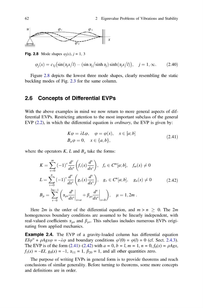
Figure 2.8 depicts the lowest three mode shapes, clearly resembling the static
buckling modes of Fig. 2.3 for the same column.
2.6 Concepts of Differential EVPs
With the above examples in mind we now return to more general aspects of differential EVPs. Restricting attention to the most important subclass of the general
EVP (2.2), in which the differential equation is ordinary, the EVP is given by:
Ku ¼ kLu; u ¼ uðxÞ; x 2 a; b
½ Š
B l u ¼ 0; x 2 a; b
f g;
ð2:41Þ
where the operators K, L and B l take the forms:
K ¼
X m
m¼0
ðÀ1Þ
m d
m
dx m f m ðxÞ
d
m
dx m
; f m 2 C
m
½a; bŠ; f m ðxÞ 6 ¼ 0
L ¼
X n
m¼0
ðÀ1Þ
m d
m
dx m g m ðxÞ
d
m
dx m
; g m 2 C
n
½a; bŠ; g n ðxÞ 6 ¼ 0
B l ¼
X
2mÀ1
m¼0
a lm
d
m
dx m
x¼a
þ b lm
d
m
dx m
x¼b
; l ¼ 1; 2m :
ð2:42Þ
Here 2m is the order of the differential equation, and m > n ! 0. The 2m
homogeneous boundary conditions are assumed to be linearly independent, with
real-valued coefficients a lm and b lm . This subclass includes numerous EVPs originating from applied mechanics.
Example 2.4. The EVP of a gravity-loaded column has differential equation
EIu′′ + qAgxu = –ku and boundary conditions u′(0) = u(l) = 0 (cf. Sect. 2.4.3).
The EVP is of the form (2.41)–(2.42) with a = 0, b = l, m = 1, n = 0, f 0 (x) = qAgx,
f 1 (x) = –EI, g 0 (x) = –1, a 11 = 1, b 20 = 1, and all other quantities zero.
The purpose of writing EVPs in general form is to provide theorems and reach
conclusions of similar generality. Before turning to theorems, some more concepts
and definitions are in order.
Fig. 2.8 Mode shapes u j (x), j = 1, 3
62
2 Eigenvalue Problems of Vibrations and Stability