2.5.1 Axial Vibrations of Straight Rods
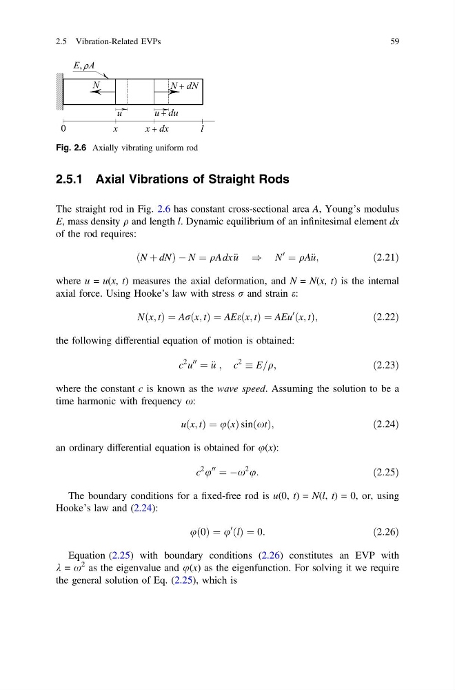
The straight rod in Fig. 2.6 has constant cross-sectional area A, Young’s modulus
E, mass density q and length l. Dynamic equilibrium of an infinitesimal element dx
of the rod requires:
ðN þ dNÞ À N ¼ qAdx€ u ) N
0
¼ qA€ u;
ð2:21Þ
where u = u(x, t) measures the axial deformation, and N = N(x, t) is the internal
axial force. Using Hooke’s law with stress r and strain e:
Nðx; tÞ ¼ Arðx; tÞ ¼ AEeðx; tÞ ¼ AEu
0
ðx; tÞ;
ð2:22Þ
the following differential equation of motion is obtained:
c
2 u
00
¼ € u ; c
2
E=q;
ð2:23Þ
where the constant c is known as the wave speed. Assuming the solution to be a
time harmonic with frequency x:
uðx; tÞ ¼ uðxÞ sinðxtÞ;
ð2:24Þ
an ordinary differential equation is obtained for u(x):
c
2 u
00
¼ Àx
2 u:
ð2:25Þ
The boundary conditions for a fixed-free rod is u(0, t) = N(l, t) = 0, or, using
Hooke’s law and (2.24):
uð0Þ ¼ u
0
ðlÞ ¼ 0:
ð2:26Þ
Equation (2.25) with boundary conditions (2.26) constitutes an EVP with
k = x
2 as the eigenvalue and u(x) as the eigenfunction. For solving it we require
the general solution of Eq. (2.25), which is
Fig. 2.6 Axially vibrating uniform rod
2.5 Vibration-Related EVPs
59