

where the implications follows from divisions by dx, and ( )′ d/dx. Differentiating
the third equation with respect to x we obtain, upon inserting the first and the
second equation, that:
M
00
À Ny
00
¼ 0:
ð2:5Þ
Since N′ = 0 and N(0) = –P, it holds that N(x) = −P. Further, according to
Hooke’s law, M(x) = EIy′′. Inserting this into (2.5) one then obtains the differential
equation governing the shape y(x) of the column:
y
0000
¼ Àky
00
; k P=EI:
ð2:6Þ
As for the boundary conditions, the three are purely geometric, while the fourth
is obtained from applying Hooke’s law to the static condition M(0)=0, thus:
yð0Þ ¼ yðlÞ ¼ y
0
ðlÞ ¼ y
00
ð0Þ ¼ 0:
ð2:7Þ
The differential Eq. (2.6) with boundary conditions (2.7) defines a differential
EVP of the general form (2.2).
Now, obviously y = 0 is a solution of (2.6) satisfying (2.7) for any value of k.
However, nontrivial solutions y 6 ¼ 0 might exist. To check this we need to solve the
EVP, which precisely means to calculate those values of k for which (2.6) with (2.7)
has nontrivial solutions y 6 ¼ 0. To solve the EVP we consider the general solution of
(2.6), which is:
yðxÞ ¼ c 1 sinðcxÞ þ c 2 cosðcxÞ þ c 3 x þ c 4 ; c
2
k;
ð2:8Þ
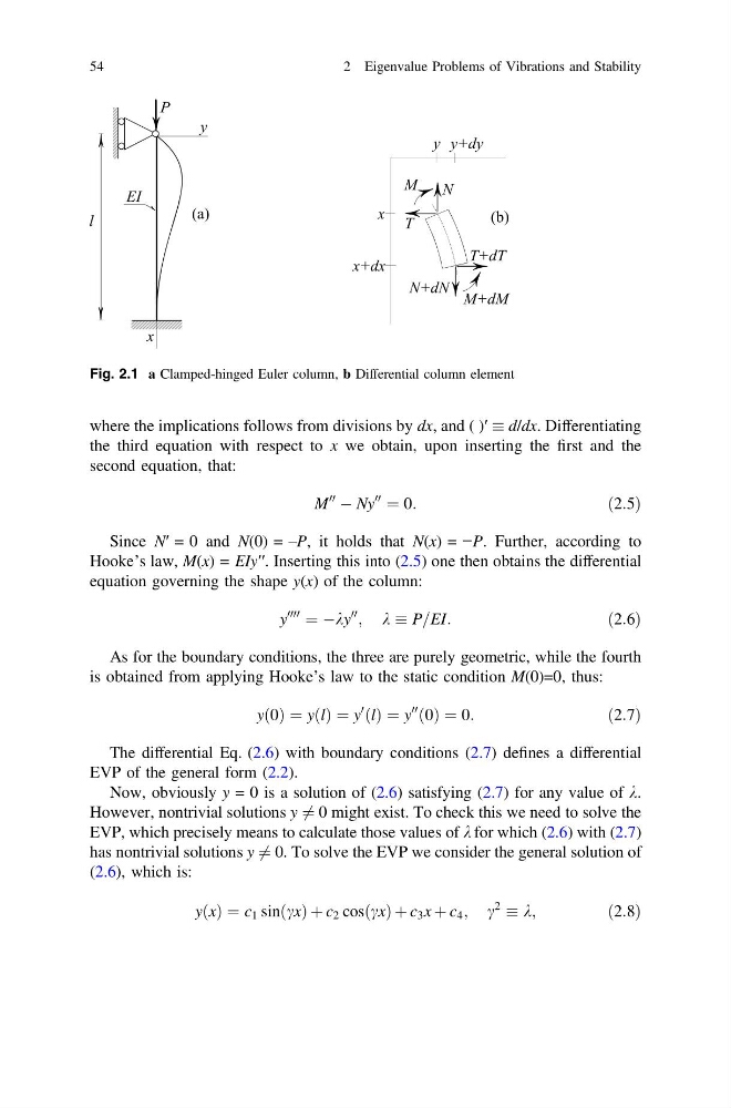
Fig. 2.1 a Clamped-hinged Euler column, b Differential column element
54
2 Eigenvalue Problems of Vibrations and Stability
the third equation with respect to x we obtain, upon inserting the first and the
second equation, that:
M
00
À Ny
00
¼ 0:
ð2:5Þ
Since N′ = 0 and N(0) = –P, it holds that N(x) = −P. Further, according to
Hooke’s law, M(x) = EIy′′. Inserting this into (2.5) one then obtains the differential
equation governing the shape y(x) of the column:
y
0000
¼ Àky
00
; k P=EI:
ð2:6Þ
As for the boundary conditions, the three are purely geometric, while the fourth
is obtained from applying Hooke’s law to the static condition M(0)=0, thus:
yð0Þ ¼ yðlÞ ¼ y
0
ðlÞ ¼ y
00
ð0Þ ¼ 0:
ð2:7Þ
The differential Eq. (2.6) with boundary conditions (2.7) defines a differential
EVP of the general form (2.2).
Now, obviously y = 0 is a solution of (2.6) satisfying (2.7) for any value of k.
However, nontrivial solutions y 6 ¼ 0 might exist. To check this we need to solve the
EVP, which precisely means to calculate those values of k for which (2.6) with (2.7)
has nontrivial solutions y 6 ¼ 0. To solve the EVP we consider the general solution of
(2.6), which is:
yðxÞ ¼ c 1 sinðcxÞ þ c 2 cosðcxÞ þ c 3 x þ c 4 ; c
2
k;
ð2:8Þ
Fig. 2.1 a Clamped-hinged Euler column, b Differential column element
54
2 Eigenvalue Problems of Vibrations and Stability