

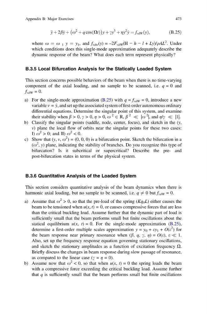
€ y þ 2b_ y þ x
2
þ q cosðXtÞ
À
Á
y þ cy
3
þ gy
2
_
y ¼ f vdW ðyÞ;
ðB:25Þ
where x x 1 y y 1 , and f vdw (y) = –2F vdW (H − h − l + Ly)/qAL
2 . Under
which conditions does this single-mode approximation adequately describe the
dynamic response of the beam? What does each term represent physically?
B.3.5 Local Bifurcation Analysis for the Statically Loaded System
This section concerns possible behaviors of the beam when there is no time-varying
component of the axial loading, and no sample to be scanned, i.e. q = 0 and
f vdW = 0.
a) For the single-mode approximation (B.25) with q = f vdW = 0, introduce a new
variable v = _
y, and set up the associated system of first-order autonomous ordinary
differential equations. Determine the singular point of this system, and examine
their stability when b > 0, c > 0, η > 0, x
2
2 R, b
2
( |x
2 |, and η/c ( |1|.
b) Classify the singular points (saddle, node, center, focus), and sketch in the (y,
v) plane the local flow of orbits near the singular points for these two cases:
I) x
2 > 0; and II) x
2 < 0.
c) Show that (y, v, x
2 ) = (0, 0, 0) is a bifurcation point. Sketch the bifurcation in a
(x
2 , y) plane, indicating the stability of branches. Do you recognize this type of
bifurcation? Is it subcritical or supercritical? Describe the pre- and
post-bifurcation states in terms of the physical system.
B.3.6 Quantitative Analysis of the Loaded System
This section considers quantitative analysis of the beam dynamics when there is
harmonic axial loading, but no sample to be scanned, i.e. q 6 ¼ 0 but f vdW = 0.
a) Assume that x
2 > 0, so that the pre-load of the spring (Kq 0 L) either causes the
beam to be tensioned when u(x, t) = 0, or causes compressive forces that are less
than the critical buckling load. Assume further that the dynamic part of load is
sufficiently small that the beam performs small but finite oscillations about the
statical equilibrium u(x, t) = 0. For the single-mode approximation (B.25),
determine a first-order multiple scales approximation y = y 0 + ey 1 + O(e
2 ) for
the beam response near primary resonance when (b, q, c, η) = O(e), e ( 1.
Also, set up the frequency response equation governing stationary oscillations,
and sketch the stationary amplitudes as a function of excitation frequency X.
Briefly discuss the changes in beam response during slow passage of resonance,
as compared to the linear case (c = η = 0).
b) Assume now that x
2 < 0, so that when u(x, t) = 0 the spring loads the beam
with a compressive force exceeding the critical buckling load. Assume further
that q is sufficiently small that the beam performs small but finite oscillations
Appendix B: Major Exercises
473
2
þ q cosðXtÞ
À
Á
y þ cy
3
þ gy
2
_
y ¼ f vdW ðyÞ;
ðB:25Þ
where x x 1 y y 1 , and f vdw (y) = –2F vdW (H − h − l + Ly)/qAL
2 . Under
which conditions does this single-mode approximation adequately describe the
dynamic response of the beam? What does each term represent physically?
B.3.5 Local Bifurcation Analysis for the Statically Loaded System
This section concerns possible behaviors of the beam when there is no time-varying
component of the axial loading, and no sample to be scanned, i.e. q = 0 and
f vdW = 0.
a) For the single-mode approximation (B.25) with q = f vdW = 0, introduce a new
variable v = _
y, and set up the associated system of first-order autonomous ordinary
differential equations. Determine the singular point of this system, and examine
their stability when b > 0, c > 0, η > 0, x
2
2 R, b
2
( |x
2 |, and η/c ( |1|.
b) Classify the singular points (saddle, node, center, focus), and sketch in the (y,
v) plane the local flow of orbits near the singular points for these two cases:
I) x
2 > 0; and II) x
2 < 0.
c) Show that (y, v, x
2 ) = (0, 0, 0) is a bifurcation point. Sketch the bifurcation in a
(x
2 , y) plane, indicating the stability of branches. Do you recognize this type of
bifurcation? Is it subcritical or supercritical? Describe the pre- and
post-bifurcation states in terms of the physical system.
B.3.6 Quantitative Analysis of the Loaded System
This section considers quantitative analysis of the beam dynamics when there is
harmonic axial loading, but no sample to be scanned, i.e. q 6 ¼ 0 but f vdW = 0.
a) Assume that x
2 > 0, so that the pre-load of the spring (Kq 0 L) either causes the
beam to be tensioned when u(x, t) = 0, or causes compressive forces that are less
than the critical buckling load. Assume further that the dynamic part of load is
sufficiently small that the beam performs small but finite oscillations about the
statical equilibrium u(x, t) = 0. For the single-mode approximation (B.25),
determine a first-order multiple scales approximation y = y 0 + ey 1 + O(e
2 ) for
the beam response near primary resonance when (b, q, c, η) = O(e), e ( 1.
Also, set up the frequency response equation governing stationary oscillations,
and sketch the stationary amplitudes as a function of excitation frequency X.
Briefly discuss the changes in beam response during slow passage of resonance,
as compared to the linear case (c = η = 0).
b) Assume now that x
2 < 0, so that when u(x, t) = 0 the spring loads the beam
with a compressive force exceeding the critical buckling load. Assume further
that q is sufficiently small that the beam performs small but finite oscillations
Appendix B: Major Exercises
473