

1.5.4 Using Lagrange’s Equations with Continuous
Systems
For continuous systems we may sometimes want to bypass setting up partial differential equations, heading on directly for an approximating set of ordinary differential equations. This can be accomplished by combining the mode shape
expansion technique described above with Lagrange’s equations, as illustrated by
the following example.
Consider again the continuous beam of Fig. 1.6, but for the purpose of illustration without the point-mass (m = 0). For setting up the equations of motion one
could employ Newton’s second law or Hamilton’s principle for obtaining the PDE,
and then turn the PDE into a set of approximating ODEs by using mode shape
expansion; this approach was used in Sect. 1.5.3. Here we choose instead to employ
mode shape expansion already at the stage of defining the energies. The expansion
(1.84) approximates the continuous variable u(x, t) in terms of a finite set of discrete
variables q j (t), j = 1, N. So, by expressing energies in terms of discrete variables q j
instead of a continuous variable u, the system transforms into a multi-DOF system.
Of course, since N needs to be finite, this system only approximates the original
continuous system. This approximation, however, would have to be introduced
anyway, we merely incorporate it at an earlier stage. The potential and kinetic
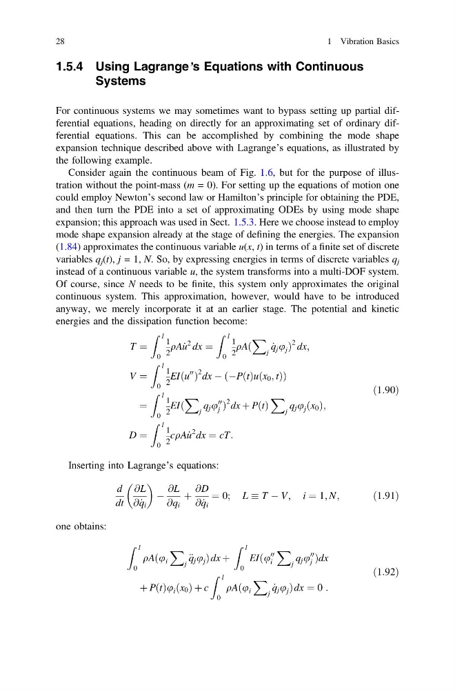
energies and the dissipation function become:
T ¼
Z l
0
1
2
qA _
u
2 dx ¼
Z l
0
1
2
qAð
X
j
_
q j u j Þ
2 dx;
V ¼
Z l
0
1
2
EIðu
00
Þ
2 dx À ÀPðtÞuðx 0 ; tÞ
ð
Þ
¼
Z l
0
1
2
EIð
X
j
q j u
00
j Þ
2 dx þ PðtÞ
X
j
q j u j ðx 0 Þ;
D ¼
Z l
0
1
2
cqA _
u
2 dx ¼ cT:
ð1:90Þ
Inserting into Lagrange’s equations:
d
dt
@L
@ _
q i
À
@L
@q i
þ
@D
@ _
q i
¼ 0; L T À V; i ¼ 1; N;
ð1:91Þ
one obtains:
Z l
0
qAðu i
X
j
€ q j u j Þdx þ
Z l
0
EIðu
00
i
X
j
q j u
00
j Þdx
þ PðtÞu i ðx 0 Þ þ c
Z l
0
qAðu i
X
j
_
q j u j Þdx ¼ 0 :
ð1:92Þ
28
1 Vibration Basics
Systems
For continuous systems we may sometimes want to bypass setting up partial differential equations, heading on directly for an approximating set of ordinary differential equations. This can be accomplished by combining the mode shape
expansion technique described above with Lagrange’s equations, as illustrated by
the following example.
Consider again the continuous beam of Fig. 1.6, but for the purpose of illustration without the point-mass (m = 0). For setting up the equations of motion one
could employ Newton’s second law or Hamilton’s principle for obtaining the PDE,
and then turn the PDE into a set of approximating ODEs by using mode shape
expansion; this approach was used in Sect. 1.5.3. Here we choose instead to employ
mode shape expansion already at the stage of defining the energies. The expansion
(1.84) approximates the continuous variable u(x, t) in terms of a finite set of discrete
variables q j (t), j = 1, N. So, by expressing energies in terms of discrete variables q j
instead of a continuous variable u, the system transforms into a multi-DOF system.
Of course, since N needs to be finite, this system only approximates the original
continuous system. This approximation, however, would have to be introduced
anyway, we merely incorporate it at an earlier stage. The potential and kinetic
energies and the dissipation function become:
T ¼
Z l
0
1
2
qA _
u
2 dx ¼
Z l
0
1
2
qAð
X
j
_
q j u j Þ
2 dx;
V ¼
Z l
0
1
2
EIðu
00
Þ
2 dx À ÀPðtÞuðx 0 ; tÞ
ð
Þ
¼
Z l
0
1
2
EIð
X
j
q j u
00
j Þ
2 dx þ PðtÞ
X
j
q j u j ðx 0 Þ;
D ¼
Z l
0
1
2
cqA _
u
2 dx ¼ cT:
ð1:90Þ
Inserting into Lagrange’s equations:
d
dt
@L
@ _
q i
À
@L
@q i
þ
@D
@ _
q i
¼ 0; L T À V; i ¼ 1; N;
ð1:91Þ
one obtains:
Z l
0
qAðu i
X
j
€ q j u j Þdx þ
Z l
0
EIðu
00
i
X
j
q j u
00
j Þdx
þ PðtÞu i ðx 0 Þ þ c
Z l
0
qAðu i
X
j
_
q j u j Þdx ¼ 0 :
ð1:92Þ
28
1 Vibration Basics