

qA
X
j
Z l
0
u i u j dx € q j þ cqA
X
j
Z l
0
u i u j dx _
q j
þ EI
X
j
Z l
0
u i u
0000
j dx q j þ PðtÞu i ðx 0 Þ ¼ 0
) qA
X
j
1
2
ld ij € q j þ cqA
X
j
1
2
ld ij _
q j
þ EI
X
j
1
2
l jp=l
ð
Þ
4 d ij q j þ PðtÞu i ðx 0 Þ ¼ 0
) qA
1
2
l€ q i þ cqA
1
2
l _
q i þ EI
1
2
l ip=l
ð
Þ
4 q i þ PðtÞu i ðx 0 Þ ¼ 0
) € q i þ c _
q i þ x
2
i q i ¼ À2ðqAlÞ
À1 PðtÞ sin ipx 0 =l
ð
Þ; i ¼ 1; N;
ð1:89Þ
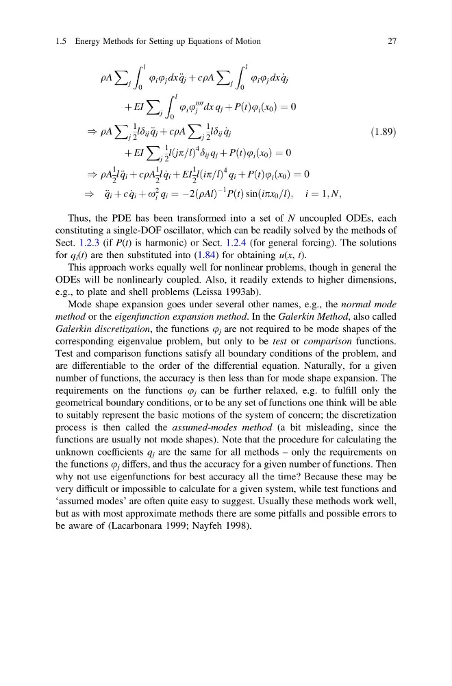
Thus, the PDE has been transformed into a set of N uncoupled ODEs, each
constituting a single-DOF oscillator, which can be readily solved by the methods of
Sect. 1.2.3 (if P(t) is harmonic) or Sect. 1.2.4 (for general forcing). The solutions
for q i (t) are then substituted into (1.84) for obtaining u(x, t).
This approach works equally well for nonlinear problems, though in general the
ODEs will be nonlinearly coupled. Also, it readily extends to higher dimensions,
e.g., to plate and shell problems (Leissa 1993ab).
Mode shape expansion goes under several other names, e.g., the normal mode
method or the eigenfunction expansion method. In the Galerkin Method, also called
Galerkin discretization, the functions u j are not required to be mode shapes of the
corresponding eigenvalue problem, but only to be test or comparison functions.
Test and comparison functions satisfy all boundary conditions of the problem, and
are differentiable to the order of the differential equation. Naturally, for a given
number of functions, the accuracy is then less than for mode shape expansion. The
requirements on the functions u j can be further relaxed, e.g. to fulfill only the
geometrical boundary conditions, or to be any set of functions one think will be able
to suitably represent the basic motions of the system of concern; the discretization
process is then called the assumed-modes method (a bit misleading, since the
functions are usually not mode shapes). Note that the procedure for calculating the
unknown coefficients q j are the same for all methods – only the requirements on
the functions u j differs, and thus the accuracy for a given number of functions. Then
why not use eigenfunctions for best accuracy all the time? Because these may be
very difficult or impossible to calculate for a given system, while test functions and
‘assumed modes’ are often quite easy to suggest. Usually these methods work well,
but as with most approximate methods there are some pitfalls and possible errors to
be aware of (Lacarbonara 1999; Nayfeh 1998).
1.5 Energy Methods for Setting up Equations of Motion
27
X
j
Z l
0
u i u j dx € q j þ cqA
X
j
Z l
0
u i u j dx _
q j
þ EI
X
j
Z l
0
u i u
0000
j dx q j þ PðtÞu i ðx 0 Þ ¼ 0
) qA
X
j
1
2
ld ij € q j þ cqA
X
j
1
2
ld ij _
q j
þ EI
X
j
1
2
l jp=l
ð
Þ
4 d ij q j þ PðtÞu i ðx 0 Þ ¼ 0
) qA
1
2
l€ q i þ cqA
1
2
l _
q i þ EI
1
2
l ip=l
ð
Þ
4 q i þ PðtÞu i ðx 0 Þ ¼ 0
) € q i þ c _
q i þ x
2
i q i ¼ À2ðqAlÞ
À1 PðtÞ sin ipx 0 =l
ð
Þ; i ¼ 1; N;
ð1:89Þ
Thus, the PDE has been transformed into a set of N uncoupled ODEs, each
constituting a single-DOF oscillator, which can be readily solved by the methods of
Sect. 1.2.3 (if P(t) is harmonic) or Sect. 1.2.4 (for general forcing). The solutions
for q i (t) are then substituted into (1.84) for obtaining u(x, t).
This approach works equally well for nonlinear problems, though in general the
ODEs will be nonlinearly coupled. Also, it readily extends to higher dimensions,
e.g., to plate and shell problems (Leissa 1993ab).
Mode shape expansion goes under several other names, e.g., the normal mode
method or the eigenfunction expansion method. In the Galerkin Method, also called
Galerkin discretization, the functions u j are not required to be mode shapes of the
corresponding eigenvalue problem, but only to be test or comparison functions.
Test and comparison functions satisfy all boundary conditions of the problem, and
are differentiable to the order of the differential equation. Naturally, for a given
number of functions, the accuracy is then less than for mode shape expansion. The
requirements on the functions u j can be further relaxed, e.g. to fulfill only the
geometrical boundary conditions, or to be any set of functions one think will be able
to suitably represent the basic motions of the system of concern; the discretization
process is then called the assumed-modes method (a bit misleading, since the
functions are usually not mode shapes). Note that the procedure for calculating the
unknown coefficients q j are the same for all methods – only the requirements on
the functions u j differs, and thus the accuracy for a given number of functions. Then
why not use eigenfunctions for best accuracy all the time? Because these may be
very difficult or impossible to calculate for a given system, while test functions and
‘assumed modes’ are often quite easy to suggest. Usually these methods work well,
but as with most approximate methods there are some pitfalls and possible errors to
be aware of (Lacarbonara 1999; Nayfeh 1998).
1.5 Energy Methods for Setting up Equations of Motion
27