

s + v can be continuous at _
z ¼ 0, even though s (and perhaps h j ) is discontinuous:
The right-hand side is calculated by averaging s (and h j ) while the velocity argument _
z þ ^
u is racing back and forth across the discontinuity – and this average may
not change much in the vicinity of _
z ¼ 0.
To set up conditions for smoothening to occur, we first note that the vector
character of the functions and their dependence on u and t is inessential for this,
since the averaging process is performed element-wise, and with u and t considered
constant. It therefore suffices to consider a general scalar function sð_ zÞ, bounded on
R, and having a single discontinuity at _
z ¼ 0, and then consider the smoothed image
~ s of s:
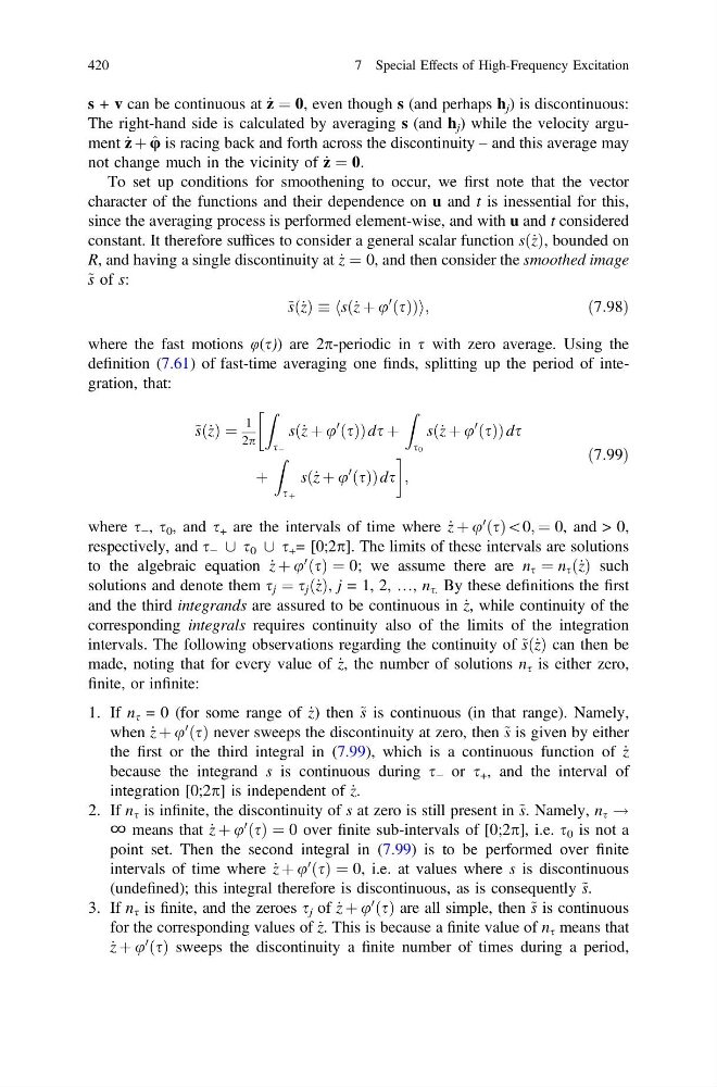
~ sð_ zÞ s _
z þ u
0
ðsÞ
ð
Þ
h
i ;
ð7:98Þ
where the fast motions φ(s)) are 2p-periodic in s with zero average. Using the
definition (7.61) of fast-time averaging one finds, splitting up the period of integration, that:
~ sð_ zÞ ¼
1
2p
Z
s À
s _
z þ u
0
ðsÞ
ð
Þds þ
Z
s 0
s _
z þ u
0
ðsÞ
ð
Þds
þ
Z
s þ
s _
z þ u
0
ðsÞ
ð
Þds
!
;
ð7:99Þ
where s − , s 0 , and s + are the intervals of time where _
z þ u
0
ðsÞ\0; ¼ 0, and > 0,
respectively, and s − [ s 0 [ s + = [0;2p]. The limits of these intervals are solutions
to the algebraic equation _
z þ u
0
ðsÞ ¼ 0; we assume there are n s ¼ n s ð_ zÞ such
solutions and denote them s j ¼ s j ð_ zÞ, j = 1, 2, …, n s. By these definitions the first
and the third integrands are assured to be continuous in _
z, while continuity of the
corresponding integrals requires continuity also of the limits of the integration
intervals. The following observations regarding the continuity of ~ sð_ zÞ can then be
made, noting that for every value of _
z, the number of solutions n s is either zero,
finite, or infinite:
1. If n s = 0 (for some range of _
z) then ~ s is continuous (in that range). Namely,
when _
z þ u
0
ðsÞ never sweeps the discontinuity at zero, then ~ s is given by either
the first or the third integral in (7.99), which is a continuous function of _
z
because the integrand s is continuous during s − or s + , and the interval of
integration [0;2p] is independent of _
z.
2. If n s is infinite, the discontinuity of s at zero is still present in ~ s. Namely, n s !
∞ means that _
z þ u
0
ðsÞ ¼ 0 over finite sub-intervals of [0;2p], i.e. s 0 is not a
point set. Then the second integral in (7.99) is to be performed over finite
intervals of time where _
z þ u
0
ðsÞ ¼ 0, i.e. at values where s is discontinuous
(undefined); this integral therefore is discontinuous, as is consequently ~ s.
3. If n s is finite, and the zeroes s j of _
z þ u
0
ðsÞ are all simple, then ~ s is continuous
for the corresponding values of _
z. This is because a finite value of n s means that
_
z þ u
0
ðsÞ sweeps the discontinuity a finite number of times during a period,
420
7 Special Effects of High-Frequency Excitation
z ¼ 0, even though s (and perhaps h j ) is discontinuous:
The right-hand side is calculated by averaging s (and h j ) while the velocity argument _
z þ ^
u is racing back and forth across the discontinuity – and this average may
not change much in the vicinity of _
z ¼ 0.
To set up conditions for smoothening to occur, we first note that the vector
character of the functions and their dependence on u and t is inessential for this,
since the averaging process is performed element-wise, and with u and t considered
constant. It therefore suffices to consider a general scalar function sð_ zÞ, bounded on
R, and having a single discontinuity at _
z ¼ 0, and then consider the smoothed image
~ s of s:
~ sð_ zÞ s _
z þ u
0
ðsÞ
ð
Þ
h
i ;
ð7:98Þ
where the fast motions φ(s)) are 2p-periodic in s with zero average. Using the
definition (7.61) of fast-time averaging one finds, splitting up the period of integration, that:
~ sð_ zÞ ¼
1
2p
Z
s À
s _
z þ u
0
ðsÞ
ð
Þds þ
Z
s 0
s _
z þ u
0
ðsÞ
ð
Þds
þ
Z
s þ
s _
z þ u
0
ðsÞ
ð
Þds
!
;
ð7:99Þ
where s − , s 0 , and s + are the intervals of time where _
z þ u
0
ðsÞ\0; ¼ 0, and > 0,
respectively, and s − [ s 0 [ s + = [0;2p]. The limits of these intervals are solutions
to the algebraic equation _
z þ u
0
ðsÞ ¼ 0; we assume there are n s ¼ n s ð_ zÞ such
solutions and denote them s j ¼ s j ð_ zÞ, j = 1, 2, …, n s. By these definitions the first
and the third integrands are assured to be continuous in _
z, while continuity of the
corresponding integrals requires continuity also of the limits of the integration
intervals. The following observations regarding the continuity of ~ sð_ zÞ can then be
made, noting that for every value of _
z, the number of solutions n s is either zero,
finite, or infinite:
1. If n s = 0 (for some range of _
z) then ~ s is continuous (in that range). Namely,
when _
z þ u
0
ðsÞ never sweeps the discontinuity at zero, then ~ s is given by either
the first or the third integral in (7.99), which is a continuous function of _
z
because the integrand s is continuous during s − or s + , and the interval of
integration [0;2p] is independent of _
z.
2. If n s is infinite, the discontinuity of s at zero is still present in ~ s. Namely, n s !
∞ means that _
z þ u
0
ðsÞ ¼ 0 over finite sub-intervals of [0;2p], i.e. s 0 is not a
point set. Then the second integral in (7.99) is to be performed over finite
intervals of time where _
z þ u
0
ðsÞ ¼ 0, i.e. at values where s is discontinuous
(undefined); this integral therefore is discontinuous, as is consequently ~ s.
3. If n s is finite, and the zeroes s j of _
z þ u
0
ðsÞ are all simple, then ~ s is continuous
for the corresponding values of _
z. This is because a finite value of n s means that
_
z þ u
0
ðsÞ sweeps the discontinuity a finite number of times during a period,
420
7 Special Effects of High-Frequency Excitation