

4. Terms of order three and higher of the Taylor-expansion of f k , do not contribute
to stiffness (to the level of approximation employed), since their gradients
vanish at the equilibrium.
5. The stiffening effect is linear, by the definition employed above. But this does
not imply that approximately correct results are always obtained by using linearized equations of motions. For example, if n = 1 and f = f(u) = sinu, then
the sum of the two terms in the parenthesis of (7.79) becomes (f′)
2 + ffʺ
p(u) = cos
2 u − sin
2 u, so that p(0) = 1, which is the same as when starting with
the linearization f(u) % u. However, if instead f(u) = cosu − 2, then one again
finds p(0) = 1, while using the linearization f(u) % −1 one finds p(0) = 0, so
that, by an otherwise appropriate linearization, the linear stiffening effect is in
this case totally overlooked. In general, referring to 2–4. above, if f contains
constant terms, then quadratic nonlinearities in u (when Taylor-expanded)
should be retained, or stiffening effects could be inadvertently overlooked.
6. The magnitude or “strength” of the stiffening effect increases linearly with the
squared RMS velocity of the excitation velocity, i.e. with the input level of
energy. Hence the particular details of the excitation time signals are unimportant for the effect, as long as the signals are periodic and have high frequency
and small amplitude. (As for the significance of the HF waveform, see also
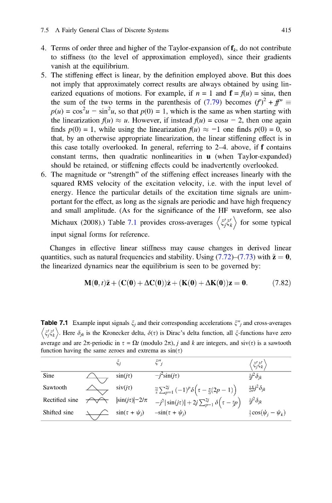
Michaux (2008).) Table 7.1 provides cross-averages n
0
j n
0
k
D
E
for some typical
input signal forms for reference.
Changes in effective linear stiffness may cause changes in derived linear
quantities, such as natural frequencies and stability. Using (7.72)–(7.73) with ~ z ¼ 0,
the linearized dynamics near the equilibrium is seen to be governed by:
Mð0; tÞ€ z þ Cð0Þ þ DCð0Þ
ð
Þ _
z þ Kð0Þ þ DKð0Þ
ð
Þ z ¼ 0:
ð7:82Þ
Table 7.1 Example input signals n j and their corresponding accelerations n′′ j and cross-averages
n
0
j n
0
k
D
E
. Here d jk is the Kronecker delta, d(s) is Dirac’s delta function, all n-functions have zero
average and are 2p-periodic in s = Xt (modulo 2p), j and k are integers, and siv(s) is a sawtooth
function having the same zeroes and extrema as sin(s)
n j
n′′ j
n
0
j n
0
k
D
E
Sine
sin(js)
−j
2
sin(js)
1
2 j
2 d jk
Sawtooth
siv(js)
2j
p
P 2j
p¼1 ðÀ1Þ
p d s À
p
2j ð2p À 1Þ
1
2
8
p 2 j
2 d jk
Rectified sine
|sin(js)|−2/p Àj
2 j sinðjsÞj þ 2j
P 2j
p¼1 d s À
p
j p
1
2 j
2 d jk
Shifted sine
sin(s + w j )
–sin(s + w j )
1
2 cosðw j À w k Þ
7.5 A Fairly General Class of Discrete Systems
415
to stiffness (to the level of approximation employed), since their gradients
vanish at the equilibrium.
5. The stiffening effect is linear, by the definition employed above. But this does
not imply that approximately correct results are always obtained by using linearized equations of motions. For example, if n = 1 and f = f(u) = sinu, then
the sum of the two terms in the parenthesis of (7.79) becomes (f′)
2 + ffʺ
p(u) = cos
2 u − sin
2 u, so that p(0) = 1, which is the same as when starting with
the linearization f(u) % u. However, if instead f(u) = cosu − 2, then one again
finds p(0) = 1, while using the linearization f(u) % −1 one finds p(0) = 0, so
that, by an otherwise appropriate linearization, the linear stiffening effect is in
this case totally overlooked. In general, referring to 2–4. above, if f contains
constant terms, then quadratic nonlinearities in u (when Taylor-expanded)
should be retained, or stiffening effects could be inadvertently overlooked.
6. The magnitude or “strength” of the stiffening effect increases linearly with the
squared RMS velocity of the excitation velocity, i.e. with the input level of
energy. Hence the particular details of the excitation time signals are unimportant for the effect, as long as the signals are periodic and have high frequency
and small amplitude. (As for the significance of the HF waveform, see also
Michaux (2008).) Table 7.1 provides cross-averages n
0
j n
0
k
D
E
for some typical
input signal forms for reference.
Changes in effective linear stiffness may cause changes in derived linear
quantities, such as natural frequencies and stability. Using (7.72)–(7.73) with ~ z ¼ 0,
the linearized dynamics near the equilibrium is seen to be governed by:
Mð0; tÞ€ z þ Cð0Þ þ DCð0Þ
ð
Þ _
z þ Kð0Þ þ DKð0Þ
ð
Þ z ¼ 0:
ð7:82Þ
Table 7.1 Example input signals n j and their corresponding accelerations n′′ j and cross-averages
n
0
j n
0
k
D
E
. Here d jk is the Kronecker delta, d(s) is Dirac’s delta function, all n-functions have zero
average and are 2p-periodic in s = Xt (modulo 2p), j and k are integers, and siv(s) is a sawtooth
function having the same zeroes and extrema as sin(s)
n j
n′′ j
n
0
j n
0
k
D
E
Sine
sin(js)
−j
2
sin(js)
1
2 j
2 d jk
Sawtooth
siv(js)
2j
p
P 2j
p¼1 ðÀ1Þ
p d s À
p
2j ð2p À 1Þ
1
2
8
p 2 j
2 d jk
Rectified sine
|sin(js)|−2/p Àj
2 j sinðjsÞj þ 2j
P 2j
p¼1 d s À
p
j p
1
2 j
2 d jk
Shifted sine
sin(s + w j )
–sin(s + w j )
1
2 cosðw j À w k Þ
7.5 A Fairly General Class of Discrete Systems
415