

As appears, Eq. (7.68) for the slow motions z is similar in form to the original
equation of motion (7.59) for the full motions u, though, with the integrated
influence of fast forces (h j + Xf j )n j ′′ accounted for by the vibrational forces v,
depending only on the slowly changing variables z and t. Any explicit dependence
on the fast time variable s = Xt has been averaged out, which makes the equation
for z far easier to solve than the original equation for u. This holds for analytical
solutions, not least because there are powerful mathematical tools applying only to
autonomous systems. And it holds for numerical solutions, where much larger time
steps can be used since there is no need to keep track of the rapid oscillations at
frequency X, and the numerical ill-posedness or ‘stiffness’ is reduced that arise
when solving systems of differential equations on vastly different time scales.
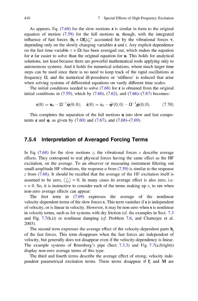
The initial conditions needed to solve (7.68) for z is obtained from the original
initial conditions in (7.59), which by (7.60), (7.62), and (7.66)–(7.67) becomes:
zð0Þ ¼ u 0 À X
À1
^
uð0; 0Þ; _
zð0Þ ¼ _
u 0 À ^
u 0 ð0; 0Þ À X
À1
^
_uð0; 0Þ:
ð7:70Þ
This completes the separation of the full motions u into slow and fast components z and φ, as given by (7.60) and (7.67), and (7.68)–(7.69).
7.5.4 Interpretation of Averaged Forcing Terms
In Eq. (7.68) for the slow motions z, the vibrational forces v describe average
effects. They correspond to real physical forces having the same effect as the HF
excitation, on the average. To an observer or measuring instrument filtering out
small-amplitude HF vibrations, the response u from (7.59) is similar to the response
z from (7.68). It should be recalled that the average of the HF excitation itself is
assumed to be zero, n j
¼ 0. In many cases its average effect is also zero, i.e.
v = 0. So, it is instructive to consider each of the terms making up v, to see when
non-zero average effects can appear:
The first term in (7.69) expresses the average of the nonlinear
velocity-dependent terms of the slow forces s. This term vanishes if s is independent
of velocity, or is linear in velocity. However, it may be non-zero when s is nonlinear
in velocity terms, such as for systems with dry friction (cf. the examples in Sect. 7.3
and Fig. 7.7(h,i)) or nonlinear damping (cf. Problem 7.6, and Chatterjee et al.
2003).
The second term expresses the average effect of the velocity-dependent parts h j
of the fast forces. This term disappears when the fast forces are independent of
velocity, but generally does not disappear even if the velocity-dependency is linear.
The example systems of Brumberg’s pipe (Sect. 7.3.3) and Fig. 7.7(a,f(right))
display non-zero average terms of this type.
The third and fourth terms describe the average effect of strong, velocity independent parametrical excitation terms. These terms disappear if f j and M are
410
7 Special Effects of High-Frequency Excitation
equation of motion (7.59) for the full motions u, though, with the integrated
influence of fast forces (h j + Xf j )n j ′′ accounted for by the vibrational forces v,
depending only on the slowly changing variables z and t. Any explicit dependence
on the fast time variable s = Xt has been averaged out, which makes the equation
for z far easier to solve than the original equation for u. This holds for analytical
solutions, not least because there are powerful mathematical tools applying only to
autonomous systems. And it holds for numerical solutions, where much larger time
steps can be used since there is no need to keep track of the rapid oscillations at
frequency X, and the numerical ill-posedness or ‘stiffness’ is reduced that arise
when solving systems of differential equations on vastly different time scales.
The initial conditions needed to solve (7.68) for z is obtained from the original
initial conditions in (7.59), which by (7.60), (7.62), and (7.66)–(7.67) becomes:
zð0Þ ¼ u 0 À X
À1
^
uð0; 0Þ; _
zð0Þ ¼ _
u 0 À ^
u 0 ð0; 0Þ À X
À1
^
_uð0; 0Þ:
ð7:70Þ
This completes the separation of the full motions u into slow and fast components z and φ, as given by (7.60) and (7.67), and (7.68)–(7.69).
7.5.4 Interpretation of Averaged Forcing Terms
In Eq. (7.68) for the slow motions z, the vibrational forces v describe average
effects. They correspond to real physical forces having the same effect as the HF
excitation, on the average. To an observer or measuring instrument filtering out
small-amplitude HF vibrations, the response u from (7.59) is similar to the response
z from (7.68). It should be recalled that the average of the HF excitation itself is
assumed to be zero, n j
¼ 0. In many cases its average effect is also zero, i.e.
v = 0. So, it is instructive to consider each of the terms making up v, to see when
non-zero average effects can appear:
The first term in (7.69) expresses the average of the nonlinear
velocity-dependent terms of the slow forces s. This term vanishes if s is independent
of velocity, or is linear in velocity. However, it may be non-zero when s is nonlinear
in velocity terms, such as for systems with dry friction (cf. the examples in Sect. 7.3
and Fig. 7.7(h,i)) or nonlinear damping (cf. Problem 7.6, and Chatterjee et al.
2003).
The second term expresses the average effect of the velocity-dependent parts h j
of the fast forces. This term disappears when the fast forces are independent of
velocity, but generally does not disappear even if the velocity-dependency is linear.
The example systems of Brumberg’s pipe (Sect. 7.3.3) and Fig. 7.7(a,f(right))
display non-zero average terms of this type.
The third and fourth terms describe the average effect of strong, velocity independent parametrical excitation terms. These terms disappear if f j and M are
410
7 Special Effects of High-Frequency Excitation