

Mðu; tÞ
d
2
u
dt 2 þ sðu;
du
dt
; tÞ þ
X m
j¼1
h j ðu;
du
dt
; tÞ þ Xf j ðu; tÞ
@
2
@ðXtÞ
2
n j ðt; XtÞ ¼ 0;
u ¼ uðtÞ; uð0Þ ¼ u 0 ;
du=dt
ð
Þ t¼0 ¼ _
u 0 ; X ) 1;
ð7:59Þ
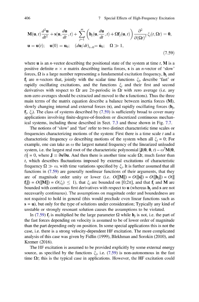
where u is an n-vector describing the positional state of the system at time t, M is a
positive definite n  n matrix describing inertia forces, s is an n-vector of ‘slow’
forces, X is a large number representing a fundamental excitation frequency, h j and
f j are n-vectors that, jointly with the scalar time functions n j , describe ‘fast’ or
rapidly oscillating excitations, and the functions n j and their first and second
derivatives with respect to Xt are 2p-periodic in Xt with zero average (i.e. any
non-zero averages should be extracted and moved to the s functions). Thus the three
main terms of the matrix equation describe a balance between inertia forces (M),
slowly changing internal and external forces (s), and rapidly oscillating forces (h j ,
f j , n j ). The class of systems described by (7.59) is sufficiently broad to cover many
applications involving finite-degree-of-freedom or discretized continuous mechanical systems, including those described in Sect. 7.3 and those shown in Fig. 7.7.
The notions of ‘slow’ and ‘fast’ refer to two distinct characteristic time scales or
frequencies characterizing motions of the system: First there is a time scale t and a
characteristic frequency x describing motions of the system when all n j = 0; For
example, one can take as x the largest natural frequency of the linearized unloaded
system, i.e. the largest real root of the characteristic polynomial |J(0, 0, t) – x
2
M(0,
t)| = 0, where J ∂s/∂u. And then there is another time scale Xt, much faster than
t, which describes fluctuations imposed by external excitations of characteristic
frequency X ) x, with time variations specified by n j . It is further assumed that all
functions in (7.59) are generally nonlinear functions of their arguments, that they
are of magnitude order unity or lower (i.e. O(||M||) = O(||s||) = O(||h j ||) = O(||
f j ||) = O(||M||) = O(n j )
1), that n j are bounded on [0;2p], and that f j and M are
bounded with continuous first derivatives with respect to u (whereas h j and s are not
necessarily continuous). The assumptions on magnitude order and boundedness are
not required to hold in general (this would preclude even linear functions such as
s = u), but only for the type of solutions under consideration; Typically any kind of
unstable or strongly resonant solution causes the assumptions to be violated.
In (7.59) f j is multiplied be the large parameter X while h j is not, i.e. the part of
the fast forces depending on velocity is assumed to be of lower order of magnitude
than the part depending only on position. In some special applications this is not the
case, i.e. there is a strong velocity-dependent HF excitation. The more complicated
analysis of this case was given by Fidlin (1999), Blekhman and Sorokin (2010), and
Kremer (2016).
The HF excitation is assumed to be provided explicitly by some external energy
source, as specified by the functions n j , i.e. (7.59) is non-autonomous in the fast
time Xt; this is the typical case in applications. However, the HF excitation could
406
7 Special Effects of High-Frequency Excitation
d
2
u
dt 2 þ sðu;
du
dt
; tÞ þ
X m
j¼1
h j ðu;
du
dt
; tÞ þ Xf j ðu; tÞ
@
2
@ðXtÞ
2
n j ðt; XtÞ ¼ 0;
u ¼ uðtÞ; uð0Þ ¼ u 0 ;
du=dt
ð
Þ t¼0 ¼ _
u 0 ; X ) 1;
ð7:59Þ
where u is an n-vector describing the positional state of the system at time t, M is a
positive definite n  n matrix describing inertia forces, s is an n-vector of ‘slow’
forces, X is a large number representing a fundamental excitation frequency, h j and
f j are n-vectors that, jointly with the scalar time functions n j , describe ‘fast’ or
rapidly oscillating excitations, and the functions n j and their first and second
derivatives with respect to Xt are 2p-periodic in Xt with zero average (i.e. any
non-zero averages should be extracted and moved to the s functions). Thus the three
main terms of the matrix equation describe a balance between inertia forces (M),
slowly changing internal and external forces (s), and rapidly oscillating forces (h j ,
f j , n j ). The class of systems described by (7.59) is sufficiently broad to cover many
applications involving finite-degree-of-freedom or discretized continuous mechanical systems, including those described in Sect. 7.3 and those shown in Fig. 7.7.
The notions of ‘slow’ and ‘fast’ refer to two distinct characteristic time scales or
frequencies characterizing motions of the system: First there is a time scale t and a
characteristic frequency x describing motions of the system when all n j = 0; For
example, one can take as x the largest natural frequency of the linearized unloaded
system, i.e. the largest real root of the characteristic polynomial |J(0, 0, t) – x
2
M(0,
t)| = 0, where J ∂s/∂u. And then there is another time scale Xt, much faster than
t, which describes fluctuations imposed by external excitations of characteristic
frequency X ) x, with time variations specified by n j . It is further assumed that all
functions in (7.59) are generally nonlinear functions of their arguments, that they
are of magnitude order unity or lower (i.e. O(||M||) = O(||s||) = O(||h j ||) = O(||
f j ||) = O(||M||) = O(n j )
1), that n j are bounded on [0;2p], and that f j and M are
bounded with continuous first derivatives with respect to u (whereas h j and s are not
necessarily continuous). The assumptions on magnitude order and boundedness are
not required to hold in general (this would preclude even linear functions such as
s = u), but only for the type of solutions under consideration; Typically any kind of
unstable or strongly resonant solution causes the assumptions to be violated.
In (7.59) f j is multiplied be the large parameter X while h j is not, i.e. the part of
the fast forces depending on velocity is assumed to be of lower order of magnitude
than the part depending only on position. In some special applications this is not the
case, i.e. there is a strong velocity-dependent HF excitation. The more complicated
analysis of this case was given by Fidlin (1999), Blekhman and Sorokin (2010), and
Kremer (2016).
The HF excitation is assumed to be provided explicitly by some external energy
source, as specified by the functions n j , i.e. (7.59) is non-autonomous in the fast
time Xt; this is the typical case in applications. However, the HF excitation could
406
7 Special Effects of High-Frequency Excitation