

With parametric excitation the pendulum equation may take the form studied in
Chap. 3:
€ h þ 2bx 0 _
h þ x
2
0 À qX
2 cosðXtÞ
À
Á
sin h ¼ 0;
ð6:51Þ
which models a pendulum with a periodically displaced support (Fig. 3.5).
In Chap. 3 a local perturbation analysis for (6.51) provided the frequency
response plot shown in Fig. 3.10. Checking the analytical results, by numerical
simulation or laboratory experiments, you will find fair agreement within the
interval of primary parametric resonance (X % 2x 0 ) only when the amplitude of
rotation is not too large. For example, if in a laboratory experiment the excitation
frequency X is swept through the range of Fig. 3.10, the observed response will
follow the theoretical curve until the amplitude comes close to p/2. The motion then
turns strongly chaotic
6 .
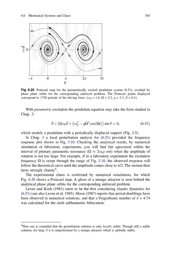
The experimental chaos is confirmed by numerical simulations, for which
Fig. 6.20 shows a Poincaré map. A ghost of a strange attractor is seen behind the
analytical phase plane orbits for the corresponding unforced problem.
Leven and Koch (1981) seem to be the first considering chaotic dynamics for
(6.51) (see also Leven et al. 1985). Moon (1987) reports that period-doublings have
been observed in numerical solutions, and that a Feigenbaum number of d = 4.74
was calculated for the sixth subharmonic bifurcation.
Fig. 6.20 Poincaré map for the parametrically excited pendulum system (6.51), overlaid by
phase plane orbits for the corresponding unforced problem. The Poincaré points displayed
correspond to 1750 periods of the driving force. (x 0 = 1.0, X = 2.2, q = 3.3, b = 0.1)
6
Thus one is reminded that the perturbation solution is only locally stable. Though still a stable
solution, for large h it is outperformed by a strange attractor which is globally stable.
6.6 Mechanical Systems and Chaos
365
Chap. 3:
€ h þ 2bx 0 _
h þ x
2
0 À qX
2 cosðXtÞ
À
Á
sin h ¼ 0;
ð6:51Þ
which models a pendulum with a periodically displaced support (Fig. 3.5).
In Chap. 3 a local perturbation analysis for (6.51) provided the frequency
response plot shown in Fig. 3.10. Checking the analytical results, by numerical
simulation or laboratory experiments, you will find fair agreement within the
interval of primary parametric resonance (X % 2x 0 ) only when the amplitude of
rotation is not too large. For example, if in a laboratory experiment the excitation
frequency X is swept through the range of Fig. 3.10, the observed response will
follow the theoretical curve until the amplitude comes close to p/2. The motion then
turns strongly chaotic
6 .
The experimental chaos is confirmed by numerical simulations, for which
Fig. 6.20 shows a Poincaré map. A ghost of a strange attractor is seen behind the
analytical phase plane orbits for the corresponding unforced problem.
Leven and Koch (1981) seem to be the first considering chaotic dynamics for
(6.51) (see also Leven et al. 1985). Moon (1987) reports that period-doublings have
been observed in numerical solutions, and that a Feigenbaum number of d = 4.74
was calculated for the sixth subharmonic bifurcation.
Fig. 6.20 Poincaré map for the parametrically excited pendulum system (6.51), overlaid by
phase plane orbits for the corresponding unforced problem. The Poincaré points displayed
correspond to 1750 periods of the driving force. (x 0 = 1.0, X = 2.2, q = 3.3, b = 0.1)
6
Thus one is reminded that the perturbation solution is only locally stable. Though still a stable
solution, for large h it is outperformed by a strange attractor which is globally stable.
6.6 Mechanical Systems and Chaos
365