

€ x þ b_ x þ
@V
@x
¼ p cosðXtÞ:
ð6:33Þ
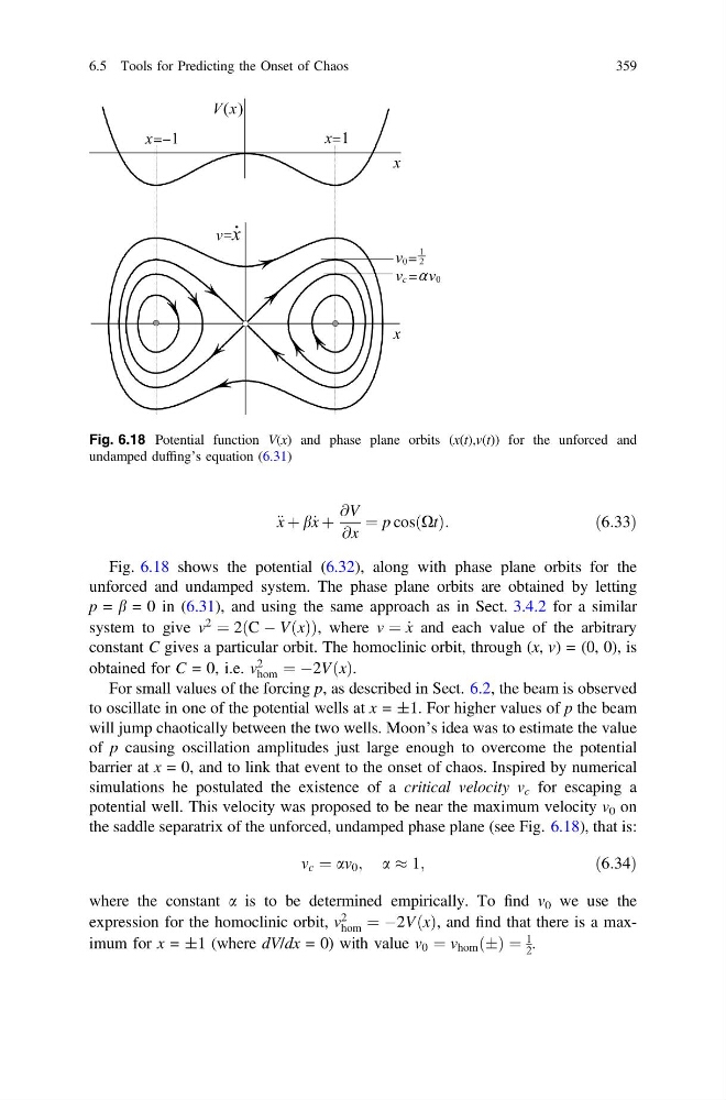
Fig. 6.18 shows the potential (6.32), along with phase plane orbits for the
unforced and undamped system. The phase plane orbits are obtained by letting
p = b = 0 in (6.31), and using the same approach as in Sect. 3.4.2 for a similar
system to give v
2
¼ 2ðC À VðxÞÞ, where v ¼ _
x and each value of the arbitrary
constant C gives a particular orbit. The homoclinic orbit, through (x, v) = (0, 0), is
obtained for C = 0, i.e. v
2
hom ¼ À2VðxÞ.
For small values of the forcing p, as described in Sect. 6.2, the beam is observed
to oscillate in one of the potential wells at x = ±1. For higher values of p the beam
will jump chaotically between the two wells. Moon’s idea was to estimate the value
of p causing oscillation amplitudes just large enough to overcome the potential
barrier at x = 0, and to link that event to the onset of chaos. Inspired by numerical
simulations he postulated the existence of a critical velocity v c for escaping a
potential well. This velocity was proposed to be near the maximum velocity v 0 on
the saddle separatrix of the unforced, undamped phase plane (see Fig. 6.18), that is:
v c ¼ av 0 ; a % 1;
ð6:34Þ
where the constant a is to be determined empirically. To find v 0 we use the
expression for the homoclinic orbit, v
2
hom ¼ À2VðxÞ, and find that there is a maximum for x = ±1 (where dV/dx = 0) with value v 0 ¼ v hom ðÆÞ ¼
1
2 .
Fig. 6.18 Potential function V(x) and phase plane orbits (x(t),v(t)) for the unforced and
undamped duffing’s equation (6.31)
6.5 Tools for Predicting the Onset of Chaos
359
@V
@x
¼ p cosðXtÞ:
ð6:33Þ
Fig. 6.18 shows the potential (6.32), along with phase plane orbits for the
unforced and undamped system. The phase plane orbits are obtained by letting
p = b = 0 in (6.31), and using the same approach as in Sect. 3.4.2 for a similar
system to give v
2
¼ 2ðC À VðxÞÞ, where v ¼ _
x and each value of the arbitrary
constant C gives a particular orbit. The homoclinic orbit, through (x, v) = (0, 0), is
obtained for C = 0, i.e. v
2
hom ¼ À2VðxÞ.
For small values of the forcing p, as described in Sect. 6.2, the beam is observed
to oscillate in one of the potential wells at x = ±1. For higher values of p the beam
will jump chaotically between the two wells. Moon’s idea was to estimate the value
of p causing oscillation amplitudes just large enough to overcome the potential
barrier at x = 0, and to link that event to the onset of chaos. Inspired by numerical
simulations he postulated the existence of a critical velocity v c for escaping a
potential well. This velocity was proposed to be near the maximum velocity v 0 on
the saddle separatrix of the unforced, undamped phase plane (see Fig. 6.18), that is:
v c ¼ av 0 ; a % 1;
ð6:34Þ
where the constant a is to be determined empirically. To find v 0 we use the
expression for the homoclinic orbit, v
2
hom ¼ À2VðxÞ, and find that there is a maximum for x = ±1 (where dV/dx = 0) with value v 0 ¼ v hom ðÆÞ ¼
1
2 .
Fig. 6.18 Potential function V(x) and phase plane orbits (x(t),v(t)) for the unforced and
undamped duffing’s equation (6.31)
6.5 Tools for Predicting the Onset of Chaos
359