

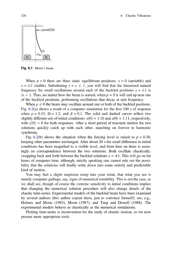
When p = 0 there are three static equilibrium positions: x = 0 (unstable) and
x = ±1 (stable). Substituting y = x Ç 1, you will find that the linearized natural
frequency for small oscillations around each of the buckled positions x = ±1 is
~
x ¼ 1. Thus, no matter how the beam is started, when p = 0 it will end up near one
of the buckled positions, performing oscillations that decay at unit frequency.
When p 6 ¼ 0 the beam may oscillate around one or both of the buckled positions.
Fig. 6.2(a) shows a result of a computer simulation for the first 100 s of response
when p = 0.15, X = 1.2, and b = 0.1. The solid and dashed curves reflect two
slightly different sets of initial conditions: x(0) = 1.10 and x(0) = 1.11, respectively,
with _
xð0Þ ¼ 0 for both responses. After a short period of transient motion the two
solutions quickly catch up with each other, marching on forever in harmonic
synchrony.
Fig. 6.2(b) shows the situation when the forcing level is raised to p = 0.30,
keeping other parameters unchanged. After about 20 s the small difference in initial
conditions has been magnified to a visible level, and from here on there is seemingly no correspondence between the two solutions. Both oscillate chaotically,
swapping back and forth between the buckled solutions x = ±1. This will go on for
hours of computer time, although, strictly speaking one cannot rule out the possibility that the solutions will finally settle down into some orderly and predictable
kind of motion.
You may feel a slight suspicion creep into your mind, that what you see is
merely computer garbage, say, signs of numerical instability. This is not the case, as
we shall see, though of course the extreme sensitivity to initial conditions implies
that changing the numerical solution procedure will also change details of the
chaotic time-series. Experimental models of the buckled beam have been examined
by several authors (this author copied them, just to convince himself); see, e.g.,
Holmes and Moon (1983), Moon (1987), and Tang and Dowell (1988). The
experimental models behave as chaotically as the numerical simulations.
Plotting time-series is inconvenient for the study of chaotic motion, so we now
present more appropriate tools.
Fig. 6.1 Moon’s beam
326
6 Chaotic Vibrations
x = ±1 (stable). Substituting y = x Ç 1, you will find that the linearized natural
frequency for small oscillations around each of the buckled positions x = ±1 is
~
x ¼ 1. Thus, no matter how the beam is started, when p = 0 it will end up near one
of the buckled positions, performing oscillations that decay at unit frequency.
When p 6 ¼ 0 the beam may oscillate around one or both of the buckled positions.
Fig. 6.2(a) shows a result of a computer simulation for the first 100 s of response
when p = 0.15, X = 1.2, and b = 0.1. The solid and dashed curves reflect two
slightly different sets of initial conditions: x(0) = 1.10 and x(0) = 1.11, respectively,
with _
xð0Þ ¼ 0 for both responses. After a short period of transient motion the two
solutions quickly catch up with each other, marching on forever in harmonic
synchrony.
Fig. 6.2(b) shows the situation when the forcing level is raised to p = 0.30,
keeping other parameters unchanged. After about 20 s the small difference in initial
conditions has been magnified to a visible level, and from here on there is seemingly no correspondence between the two solutions. Both oscillate chaotically,
swapping back and forth between the buckled solutions x = ±1. This will go on for
hours of computer time, although, strictly speaking one cannot rule out the possibility that the solutions will finally settle down into some orderly and predictable
kind of motion.
You may feel a slight suspicion creep into your mind, that what you see is
merely computer garbage, say, signs of numerical instability. This is not the case, as
we shall see, though of course the extreme sensitivity to initial conditions implies
that changing the numerical solution procedure will also change details of the
chaotic time-series. Experimental models of the buckled beam have been examined
by several authors (this author copied them, just to convince himself); see, e.g.,
Holmes and Moon (1983), Moon (1987), and Tang and Dowell (1988). The
experimental models behave as chaotically as the numerical simulations.
Plotting time-series is inconvenient for the study of chaotic motion, so we now
present more appropriate tools.
Fig. 6.1 Moon’s beam
326
6 Chaotic Vibrations