

5.14.4 The Partially Follower-loaded Double
Pendulum
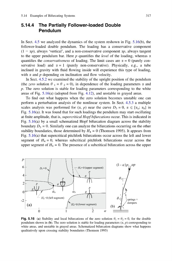
In Sect. 4.5 we analyzed the dynamics of the system reshown in Fig. 5.16(b), the
follower-loaded double pendulum. The loading has a conservative component
(1 − ap), always ‘vertical’, and a non-conservative component ap, always tangent
to the upper pendulum bar. Here p quantifies the level of the loading, whereas a
quantifies the conservativeness of loading. The limit cases are a = 0 (purely conservative load) and a = 1 (purely non-conservative). Physically, e.g., a tube
inclined in gravity with fluid flowing inside will experience this type of loading,
with a and p depending on inclination and flow velocity.
In Sect. 4.5.2 we examined the stability of the upright position of the pendulum
(the zero solution h 1 = h 2 = 0), in dependence of the loading parameters a and
p. The zero solution is stable for loading parameters corresponding to the white
areas of Fig. 5.16(a) (adopted from Fig. 4.12), and unstable in grayed areas.
To find out what happens when the zero solution becomes unstable one can
perform a perturbation analysis of the nonlinear system. In Sect. 4.5.3 a multiple
scales analysis was performed for (a, p) near the curve D 3 = 0, a 2 [a a ; a b ] in
Fig. 5.16(a). It was found that for such loadings the pendulum may start oscillating
at finite amplitude, that is, supercritical Hopf bifurcations occur. This is indicated in
Fig. 5.16(a) by a small schematized Hopf bifurcation diagram across the stability
boundary D 3 = 0. Similarly one can analyze the bifurcations occurring on the other
stability boundaries, those determined by H 4 = 0 (Thomsen 1995). It appears from
Fig. 5.16(a) that supercritical pitchfork bifurcations occur across the left and lower
segment of H 4 = 0, whereas subcritical pitchfork bifurcations occur across the
upper segment of H 4 = 0. The presence of a subcritical bifurcation across the upper
Fig. 5.16 (a) Stability and local bifurcations of the zero solution h 1 = h 2 = 0, for the double
pendulum shown in (b). The zero solution is stable for loading parameters (a, p) corresponding to
white areas, and unstable in grayed areas. Schematized bifurcation diagrams show what happens
qualitatively upon crossing stability boundaries (Thomsen 1995)
5.14 Examples of Bifurcating Systems
317
Pendulum
In Sect. 4.5 we analyzed the dynamics of the system reshown in Fig. 5.16(b), the
follower-loaded double pendulum. The loading has a conservative component
(1 − ap), always ‘vertical’, and a non-conservative component ap, always tangent
to the upper pendulum bar. Here p quantifies the level of the loading, whereas a
quantifies the conservativeness of loading. The limit cases are a = 0 (purely conservative load) and a = 1 (purely non-conservative). Physically, e.g., a tube
inclined in gravity with fluid flowing inside will experience this type of loading,
with a and p depending on inclination and flow velocity.
In Sect. 4.5.2 we examined the stability of the upright position of the pendulum
(the zero solution h 1 = h 2 = 0), in dependence of the loading parameters a and
p. The zero solution is stable for loading parameters corresponding to the white
areas of Fig. 5.16(a) (adopted from Fig. 4.12), and unstable in grayed areas.
To find out what happens when the zero solution becomes unstable one can
perform a perturbation analysis of the nonlinear system. In Sect. 4.5.3 a multiple
scales analysis was performed for (a, p) near the curve D 3 = 0, a 2 [a a ; a b ] in
Fig. 5.16(a). It was found that for such loadings the pendulum may start oscillating
at finite amplitude, that is, supercritical Hopf bifurcations occur. This is indicated in
Fig. 5.16(a) by a small schematized Hopf bifurcation diagram across the stability
boundary D 3 = 0. Similarly one can analyze the bifurcations occurring on the other
stability boundaries, those determined by H 4 = 0 (Thomsen 1995). It appears from
Fig. 5.16(a) that supercritical pitchfork bifurcations occur across the left and lower
segment of H 4 = 0, whereas subcritical pitchfork bifurcations occur across the
upper segment of H 4 = 0. The presence of a subcritical bifurcation across the upper
Fig. 5.16 (a) Stability and local bifurcations of the zero solution h 1 = h 2 = 0, for the double
pendulum shown in (b). The zero solution is stable for loading parameters (a, p) corresponding to
white areas, and unstable in grayed areas. Schematized bifurcation diagrams show what happens
qualitatively upon crossing stability boundaries (Thomsen 1995)
5.14 Examples of Bifurcating Systems
317